the Creative Commons Attribution 4.0 License.
the Creative Commons Attribution 4.0 License.
 | 11 Jun 2021
Automated quantification of floating wood pieces in rivers from video monitoring: a new software tool and validation
Hossein Ghaffarian
Pierre Lemaire
Zhang Zhi
Laure Tougne
Bruce MacVicar
Hervé Piégay
Wood is an essential component of rivers and plays a significant role in ecology and morphology. It can be also considered a risk factor in rivers due to its influence on erosion and flooding. Quantifying and characterizing wood fluxes in rivers during floods would improve our understanding of the key processes but are hindered by technical challenges. Among various techniques for monitoring wood in rivers, streamside videography is a powerful approach to quantify different characteristics of wood in rivers, but past research has employed a manual approach that has many limitations. In this work, we introduce new software for the automatic detection of wood pieces in rivers. We apply different image analysis techniques such as static and dynamic masks, object tracking, and object characterization to minimize false positive and missed detections. To assess the software performance, results are compared with manual detections of wood from the same videos, which was a time-consuming process. Key parameters that affect detection are assessed, including surface reflections, lighting conditions, flow discharge, wood position relative to the camera, and the length of wood pieces. Preliminary results had a 36 % rate of false positive detection, primarily due to light reflection and water waves, but post-processing reduced this rate to 15 %. The missed detection rate was 71 % of piece numbers in the preliminary result, but post-processing reduced this error to only 6.5 % of piece numbers and 13.5 % of volume. The high precision of the software shows that it can be used to massively increase the quantity of wood flux data in rivers around the world, potentially in real time. The significant impact of post-processing indicates that it is necessary to train the software in various situations (location, time span, weather conditions) to ensure reliable results. Manual wood detections and annotations for this work took over 150 labor hours. In comparison, the presented software coupled with an appropriate post-processing step performed the same task in real time (55 h) on a standard desktop computer.
- Article
(16268 KB) - Full-text XML
- BibTeX
- EndNote


Floating wood has a significant impact on river morphology (Gurnell et al., 2002; Gregory et al., 2003; Wohl, 2013; Wohl and Scott, 2017). It is both a component of stream ecosystems and a source of risk for human activities (Comiti et al., 2006; Badoux et al., 2014; Lucía et al., 2015). The deposition of wood at given locations can cause a reduction of the cross-sectional area, which can both increase upstream water levels (and the risk for neighboring communities) and laterally concentrate the flow downstream, which can lead to damaged infrastructure (Lyn et al., 2003; Zevenbergen et al., 2006; Mao and Comiti, 2010; Badoux et al., 2014; Ruiz-Villanueva et al., 2014; De Cicco et al., 2018; Mazzorana et al., 2018). Therefore, understanding and monitoring the dynamics of wood within a river are fundamental to assess and mitigate risk. An important body of work on this topic has grown over the last 2 decades, which has led to the development of many monitoring techniques (Marcus et al., 2002; MacVicar et al., 2009a; MacVicar and Piégay, 2012; Benacchio et al., 2015; Ravazzolo et al., 2015; Ruiz-Villanueva et al., 2019; Ghaffarian et al., 2020; Zhang et al., 2021) and conceptual and quantitative models (Braudrick and Grant, 2000; Martin and Benda, 2001; Abbe and Montgomery, 2003; Gregory et al., 2003; Seo and Nakamura, 2009; Seo et al., 2010). A recent review by Ruiz-Villanueva et al. (2016), however, argues that the area remains in relative infancy compared to other river processes such as the characterization of channel hydraulics and sediment transport. Many questions remain open areas of inquiry including wood hydraulics, which is needed to understand wood recruitment, movement and trapping, and wood budgeting; better parametrization is needed to understand and model the transfer of wood in watersheds at different scales.
In this domain, the quantification of wood mobility and wood fluxes in real rivers is a fundamental limitation that constrains model development. Most early works were based on repeated field surveys (Keller and Swanson, 1979; Lienkaemper and Swanson, 1987), with more recent efforts taking advantage of aerial photos or satellite images (Marcus et al., 2003; Lejot et al., 2007; Lassettre et al., 2008; Senter and Pasternack, 2011; Boivin et al., 2017) to estimate wood delivery at larger timescales of 1 year up to several decades. Others have monitored wood mobility once introduced by tracking wood movement in floods (Jacobson et al., 1999; Haga et al., 2002; Warren and Kraft, 2008). Tracking technologies such as active and passive radio frequency identification transponders (MacVicar et al., 2009a; Schenk et al., 2014) or GPS emitters and receivers (Ravazzolo et al., 2015) can improve the precision of this strategy. To better understand wood flux, specific trapping structures such as reservoirs or hydropower dams can be used to sample the flux over time interval windows (Moulin and Piégay, 2004; Seo et al., 2008; Turowski et al., 2013). Accumulations upstream of a retention structure can also be monitored where they trap most or all of the transported wood, as was observed by Boivin et al. (2015), to quantify wood flux at the flood event or annual scale. All these approaches allow the assessment of the wood budget and in-channel wood exchange between geographical compartments within a given river reach and over a given period (Schenk et al., 2014; Boivin et al., 2015, 2017).
For finer-scale information on the transport of wood during flood events, video recording of the water surface is suitable for estimating instantaneous fluxes and size distributions of floating wood in transport (Ghaffarian et al., 2020). Classic monitoring cameras installed on the riverbank are cheap and relatively easy to acquire, set up, and maintain. As is seen in Table 1, a wide range of sampling rates and spatial–temporal scales have been used to assess wood budgets in rivers. MacVicar and Piégay (2012) and Zhang et al. (2021) (in review), for instance, monitored wood fluxes at 5 frames per second (fps) and a resolution of 640 × 480 up to 800 × 600 pixels. Boivin et al. (2017) used a similar camera and frame rate as MacVicar and Piégay (2012) to compare periods of wood transport with and without the presence of ice. Senter et al. (2017) analyzed the complete daytime record of 39 d of videos recorded at 4 fps and a resolution of 2048 × 1536 pixels. Conceptually similar to the video technique, time-lapse imagery can be substituted for large rivers where surface velocities are low enough and the field of view is large. Kramer and Wohl (2014) and Kramer et al. (2017) applied this technique in the Slave River (Canada) and recorded one image every 1 and 10 min. Where possible, wood pieces within the field of view are then visually detected and measured using simple software to measure the length and diameter of the wood to estimate wood flux (pieces per second) or wood volume (m3 s−1) (MacVicar and Piégay, 2012; Senter et al., 2017). Critically for this approach, the time it takes for the researchers to extract information about wood fluxes has limited the fraction of the time that can be reasonably analyzed. Given the outdoor location for the camera, the image properties depend heavily on lighting conditions (e.g., surface light reflections, low light, ice, poor resolution, or surface waves), which may also limit the accuracy of frequency and size information (Muste et al., 2008; MacVicar et al., 2009a). In such situations, simpler metrics such as a count of wood pieces, a classification of wood transport intensity, or even just a binary presence–absence may be used to characterize the wood flux (Boivin et al., 2017; Kramer et al., 2017).
Table 1Characteristics of streamside video monitoring techniques in different studies.

A fully automatic wood detection and characterization algorithm can greatly improve our ability to exploit the vast amounts of data on wood transport that can be collected from streamside video cameras. From a computer science perspective, however, automatic detection and characterization remain challenging issues. In computer vision, detecting objects within videos typically consists of separating the foreground (the object of interest) from the background (Roussillon et al., 2009; Cerutti et al., 2011, 2013). The basic hypothesis is that the background is relatively static and covers a large part of the image, allowing it to be matched between successive images. In riverine environments, however, such an assumption is unrealistic because the background shows a flowing river, which can have rapidly fluctuating properties (Ali and Tougne, 2009). Floating objects are also partially submerged in water that has high suspended material concentrations during floods, making them only partially visible (e.g., a single piece of wood may be perceived as multiple objects) (MacVicar et al., 2009b). Detecting such an object in motion within a dynamic background is an area of active research (Ali et al., 2012, 2014; Lemaire et al., 2014; Piégay et al., 2014; Benacchio et al., 2017). Accurate object detection typically relies on the assumption that objects of a single class (e.g., faces, bicycles, animals) have a distinctive aspect or set of features that can be used to distinguish between types of objects. With the help of a representative dataset, machine-learning algorithms aim to define the most salient visual characteristics of the class of interest (Lemaire et al., 2014; Viola and Jones, 2006). When the objects have a wide intra-class aspect range, a large amount of data can compensate by allowing the application of deep learning algorithms (Gordo et al., 2016; Liu et al., 2020). To our knowledge, such a database is not available in the case of floating wood.
The camera installed on the Ain River in France has been operating more or less continuously for over 10 years, and vast improvements in data storage mean that these data can be saved indefinitely (Zhang et al., 2021). The ability to process this image database to extract the wood fluxes allows us to integrate this information over floods, seasons, and years, which would allow us to significantly advance our understanding of the variability within and between floods over a long time period. An unsupervised method to identify floating wood in these videos by applying intensity, gradient, and temporal masks was developed by Ali and Tougne (2009) and Ali et al. (2011). In this model, the objects were tracked through the frame to ensure that they followed the direction of flow. An analysis of about 35 min of the video showed that approximately 90 % of the wood pieces was detected (i.e., about 10 % of detections were missed), which confirmed the potential utility of this approach. An additional set of false detections related to surface wave conditions amounted to approximately 15 % of the total detection. However, the developed algorithm was not always stable and was found to perform poorly when applied to a larger dataset (i.e., video segments more than 1 h).
The objectives of the presented work are to describe and validate a new algorithm and computer interface for quantifying floating wood pieces in rivers. First, the algorithm procedure is introduced to show how wood pieces are detected and characterized. Second, the computer interface is presented to show how manual annotation is integrated with the algorithm to train the detection procedure. Third, the procedure is validated using data from the Ain River. The validation period occurred over 6 d in January and December 2012 when flow conditions ranged from ∼400 m3 s−1, which is below bankfull discharge but above the wood transport threshold, to more than 800 m3 s−1.
The Ain River is a piedmont river with a drainage area of 3630 km2 at the gauging station of Chazey-sur-Ain, with a mean flow width of 65 m, a mean slope of 0.15 %, and a mean annual discharge of 120 m3 s−1. The lower Ain River is characterized by an active channel shifting within a forested floodplain (Lassettre et al., 2008). An AXIS221 Day/Night™ camera with a resolution of 768 × 576 pixels was installed at this station to continuously record the water surface of the river at a maximum frequency of 5 fps (Fig. 1). This camera replaced a lower-resolution camera at the same location used by MacVicar and Piégay (2012). The specific location of the camera is on the outer bank of a meander, on the side closest to the thalweg, at a height of 9.8 m above the base flow elevation. The meander and a bridge pier upstream help to steer most of the floating wood so that it passes relatively close to the camera where it can be readily detected with a manual procedure (MacVicar and Piégay, 2012). The flow discharge is available from the website (http://www.hydro.eaufrance.fr/, last access: 1 June 2020).
The survey period examined on this river was during 2012, from which two flood events (1–7 January and 15 December) were selected for annotation. A range of discharges from 400 to 800 m3 s−1 occurred during these periods (Fig. 1e), which is above a previously observed wood transport threshold of ∼300 m3 s−1 (MacVicar and Piégay, 2012). A summary of automated and manual detections for the 6 d is shown in Table 3.
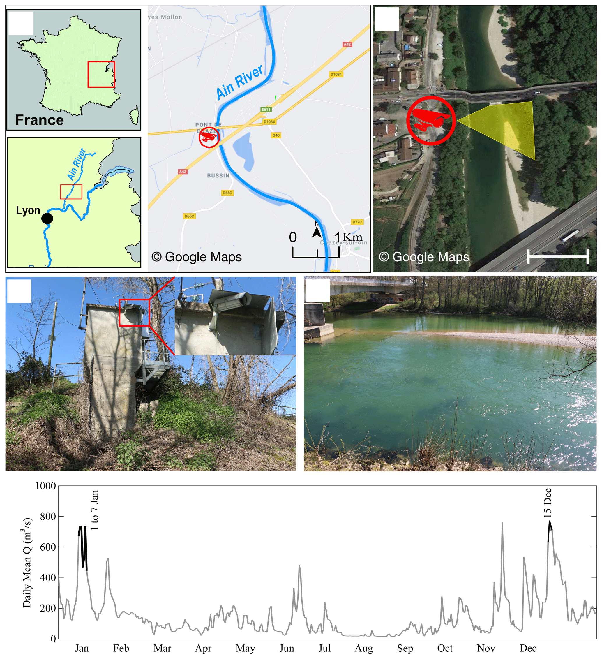
Figure 1Study site at Pont de Chazey: (a) location of the Ain River catchment in France and location of the gauging station, (b) camera position and its view angle in yellow, (c) overview of the gauging station with the camera installation point, and (d) view of the river channel from the camera. (e) Daily mean discharge series for the monitoring period from 1 to 7 January and on 15 December.
The algorithm for wood detection comprises a number of steps that seek to locate objects moving through the field of view in a series of images and then identify the objects most likely to be wood. The algorithm used in this work modifies the approach described by Ali et al. (2011). The steps work from a pixel to image to video scale, with the context from the larger scale helping to assess whether the information at the smaller scale indicates the presence of floating wood or not. In a still image, a single pixel is characterized by its location within the image, its color, and its intensity. Looking at its surrounding pixels on an image scale allows information to be spatially contextualized. Meanwhile, the video data add temporal context so that previous and future states of a given pixel can be used to assess its likeliness of representing floating wood. On a video scale, the method can embed expectations about how wood pieces should move through frames, how big they should be, and how lighting and weather conditions can evolve to change the expectations of wood appearance, location, and movement. The specific steps followed by the algorithm are shown in a simple flowchart (Fig. 2a). An example image with a wood piece in the middle of the frame is also shown for reference (Fig. 2b).
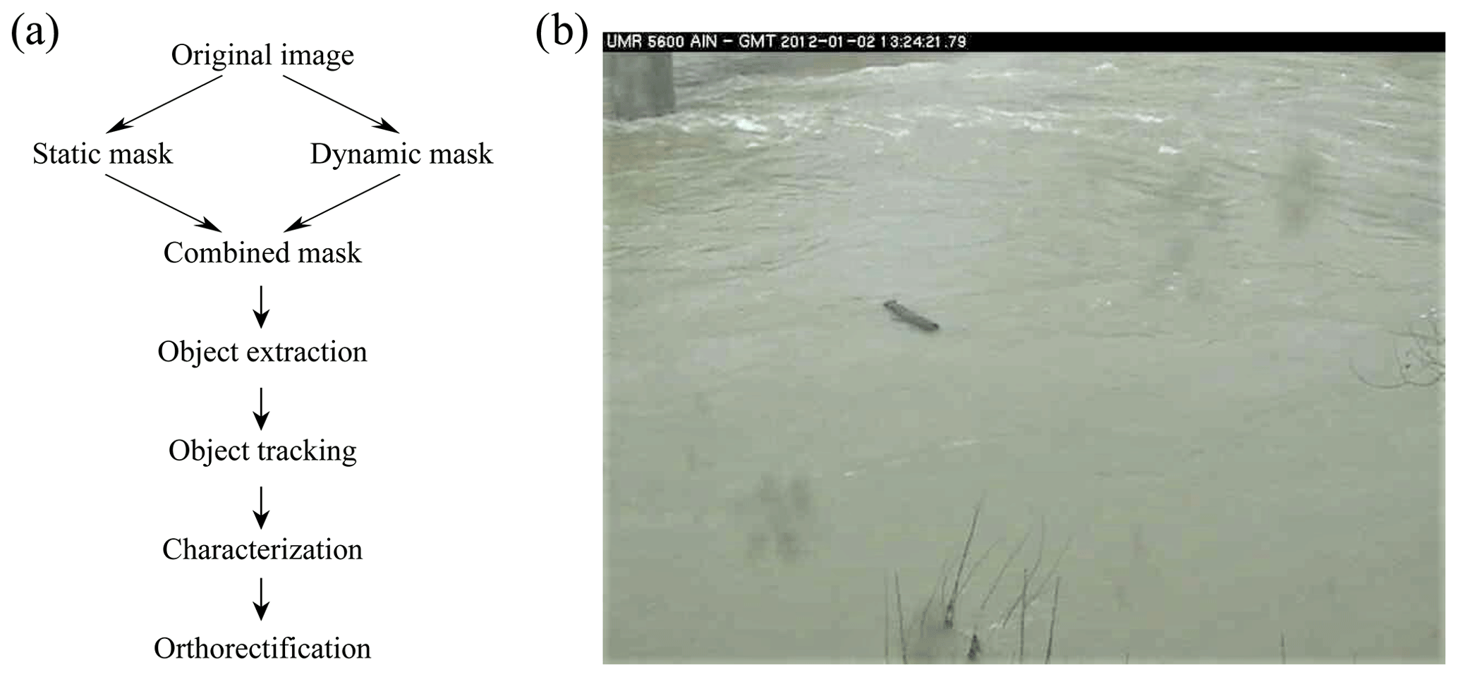
Figure 2(a) Flowchart of the detection software and (b) an example of the frame on which these different flowchart steps are applied.
3.1 Wood probability masks
In the first step, each pixel was analyzed individually and independently. The static probability mask answers the following question: is one pixel likely to belong to a wood block given its color and intensity? The algorithm assumes that the wood pixels can be identified by pixel light intensity (i) following a Gaussian distribution (Fig. 3a). To set the algorithm parameters, pixel-wise annotations of wood under all the observed lighting conditions were used to determine the mean (μ) and standard deviation (σ) of wood piece pixel intensity. Applying this algorithm produces a static probability mask (Fig. 3b). From this figure, it is possible to identify the sectors where wood presence is likely, which includes the floating wood piece seen in Fig. 2b, but also includes standing vegetation in the lower part of the image and a shadowed area in the upper left. The advantage of this approach is that it is computationally very fast. However, misclassification is possible, particularly when light conditions change.
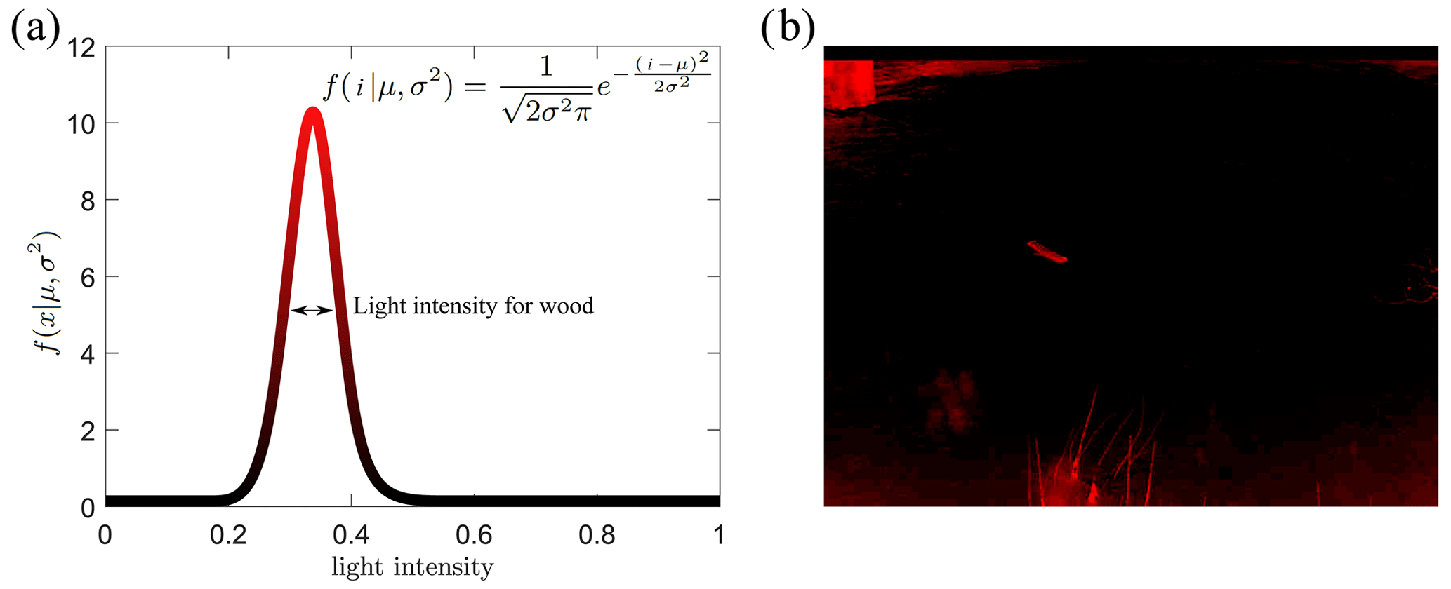
Figure 3Static probability mask, (a) Gaussian distribution of light intensity range for a piece of wood, and (b) employment of a probability mask on the sample frame.
The second mask, called the dynamic probability mask, outlines each pixel's recent history. The corresponding question is the following: is this pixel likely to represent wood now given its past and present characteristics? Again, this step is based on what is most common in our database: it is assumed that a wood pixel is darker than a water pixel. Depending on lighting conditions like shadows cast on water or waves, this is not always true; i.e., water pixels can be as dark as wood pixels. However, pixels displaying successively water then wood tend to become immediately and significantly darker, while pixels displaying wood then water tend to become significantly lighter. Meanwhile, the intensity of pixels that keep on displaying wood tends to be rather stable. Thus, we assign wood pixel probability according to an updated version of the function proposed by Ali et al. (2011) (Fig. 4a) that takes four parameters. This function H is an updating function, which produces a temporal probability mask from the inter-frame pixel value. On a probability map, a pixel value ranges from −1 (likely not wood) to 1 (likely wood). The temporal mask value for a pixel at location (xy) and at time t is PT(x,y,t)=H(Δt,I)+PT(x,y,t-1). We apply a threshold to the output of PT(x,y,t) so that it always stays within the interval [0,1]. The idea is that a pixel that becomes suddenly and significantly darker is assumed to likely be wood. H(Δt,I) is such that under those conditions, it increases the pixel probability map value (parameters τ and β). A pixel that becomes lighter over time is unlikely to correspond to wood (parameter α). A pixel for which the intensity is stable and that was previously assumed to be wood shall still correspond to wood, while a pixel for which the intensity is stable and for which the probability to be wood was low is unlikely to represent wood now. A small decay factor (δ) was introduced in order to prevent divergence (in particular, it prevents noisy areas from being activated too frequently).
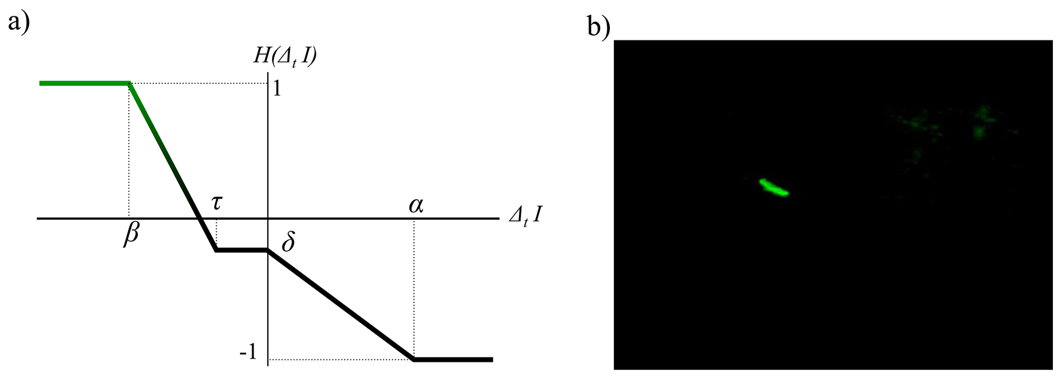
Figure 4Dynamic probability mask, (a) updating function H(Δt,I) adapted from Ali et al. (2011), and (b) employment of a probability mask on the sample frame.
The final wood probability mask is created using a combination of both the static and dynamic probability masks. Wood objects thus had to have a combination of the correct pixel color and the expected temporal behavior of water–wood–water color. The masks were combined assuming that both probabilities are independent, which allowed us to use the Bayesian probability rule in which the probability masks are simply multiplied, pixel by pixel, to obtain the final probability value for each pixel of every frame.
3.2 Wood object identification and characterization
From the probability mask it is necessary to group pixels with high wood probabilities into objects and then to separate these objects from the background to track them through the image frame. For this purpose, pixels were classified as high or low probability based on a threshold applied to the combined probability mask. Then, the high-probability pixels were grouped into connected components (that is, small, contiguous regions on the image) to define the objects. At this stage, a pixel size threshold was applied to the detected objects so that only the bigger objects were considered to represent woody objects on the water surface (Fig. 5a the big white region in the middle). A number of smaller components were often related to non-wood objects, for example waves, reflections, or noise from the camera sensor or data compression.
After the size thresholding step, movement direction and velocity were used as filters to distinguish real objects from false detections. The question here is the following: is this object moving through the image frame the way we would expect floating wood to move? To do this, the spatial and temporal behavior of components was analyzed. First, to deal with partly immersed objects, we agglomerated multiple objects within frames as components of a single object if the distance separating them was less than a set threshold. Second, we associated wood objects in successive frames together to determine if the motion of a given object was compatible with what is expected from driftwood. This can be achieved according to the dimensionless parameter PT/ΔT, which provides a general guideline for the distance an object passes between two consecutive frames (Zhang et al., 2021). Here PT (passing time) is the time that one piece of wood passes through the camera field of view, and ΔT is the time between two consecutive frames; practically, it is recommended to use videos with PT/ΔT>5 in this software. In our case, tracking wood is rather difficult for classical object tracking approaches in computer vision: the background is very noisy, the acquisition frequency is low, and the object's appearance can be highly variable due to temporarily submerged parts and highly variable 3D structures. Given these considerations it was necessary to use very basic rules for this step. The rules are therefore based on loose expectations, in terms of pixel intervals, regarding the motions of the objects depending on the camera location and the river properties. How many pixels is the object likely to move between image frames from left to right? How many pixels from top to bottom? How many appearances are required? How many frames can we miss because of temporary immersions? Using these rules, computational costs remained low and the analysis could be run in real time while also providing good performance.
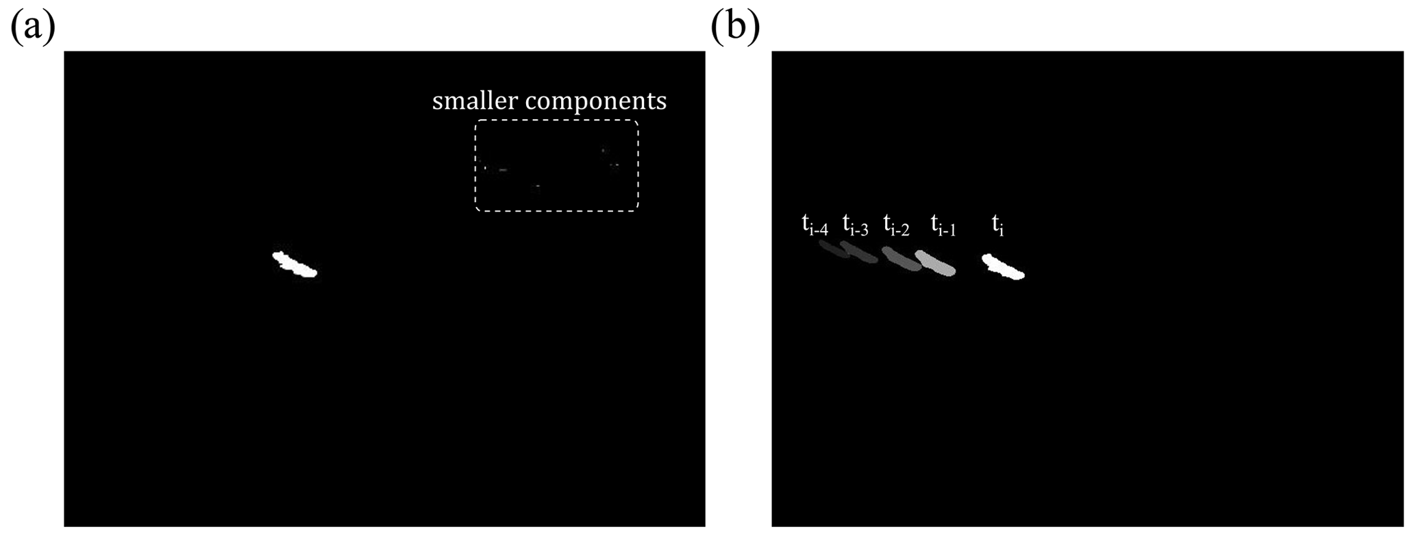
Figure 5(a) Object extraction by (i) combining static and dynamic masks and (ii) applying a threshold to retain only high-probability pixels. (b) Object tracking as a filter to deal with partly immersed objects and to distinguish moving objects from static waves.
The final step was to characterize each object which at this point in the process are considered wood objects. Each appears several times in different frames, and a procedure is needed to either pick a single representative occurrence or use a statistical tool to analyze multiple occurrences to estimate characterization data. In this step, all images containing the object are transformed from pixel to Cartesian coordinates (as will be described in the next section), and the median length is calculated and used as the most representative state. This approach also matched the manual annotation procedure whereby we tended to pick the view of the object that covers the largest area to make measurements. For the current paper, every object is characterized from the raw image based on its size and its location. It is worth saying that detection was only possible during the daylight.
3.3 Image rectification
Warping images according to a perspective transform results in an important loss of quality. On warped images, areas of the image farther from the camera provide little detail and are overall very blurry and non-informative. Therefore, image rectification was necessary to calculate wood length, velocity, and volume from the saved pixel-based characterization of each object. To do so, the fish-eye lens distortion was first corrected. A fish-eye lens distortion is a characteristic of the lens that produces visual distortion intended to create a wide panoramic or hemispherical image. This effect was corrected by a standard MATLAB process using the ComputerVisionToolbox™ (Release 2017b).
Ground-based cameras also have an oblique angle of view, which means that pixel-to-meter correspondence is variable and images need to be orthorectified to obtain estimates of object size and velocity in real terms (Muste et al., 2008). Orthorectification refers to the process by which image distortion is removed and the image scale is adjusted to match the actual scale of the water surface. Translating from pixels to Cartesian coordinates required us to assume that our camera follows the pinhole camera model and that the river can be assimilated to a plane of constant altitude. Under such conditions, it is possible to translate from pixel coordinates to a metric 2D space thanks to a perspective transform assuming a virtual pinhole camera on the image and estimating the position of the camera and its principal point (center of the view). An example of orthorectification on a detected wood piece in a set of continuous frames and pixel coordinates (Fig. 6a) is presented in Fig. 6b in metric coordinates. The transform matrix is obtained with the help of at least four non-colinear points (Fig. 6c, blue GCPs – ground control points – acquired with DGPS) from which we know both the relative 2D metric coordinates for a given water level (Fig. 6b, blue points) and their corresponding localization within the image (Fig. 6a, blue points). To achieve better accuracy, it is advised to acquire additional points and to solve the subsequent overdetermined system with the help of a least square regression (LSR). Robust estimators such as RANSAC (Forsyth and Ponce, 2012) can be useful tools to prevent acquisition noise. After identifying the virtual camera position, the perspective transform matrix then becomes parameterized with the water level. Handling the variable water level was performed for each piece of wood by measuring the relative height between the camera and the water level at the time of detection based on information recorded at the gauging station to which the camera was attached. The transformation matrix on the Ain River at the base flow elevation with the camera as the origin is shown in Fig. 6d. Straight lines near the edges of the image appear curved because the fish-eye distortion has been corrected on this image; conversely, a straight line, in reality, is presented without any curvature in the image.
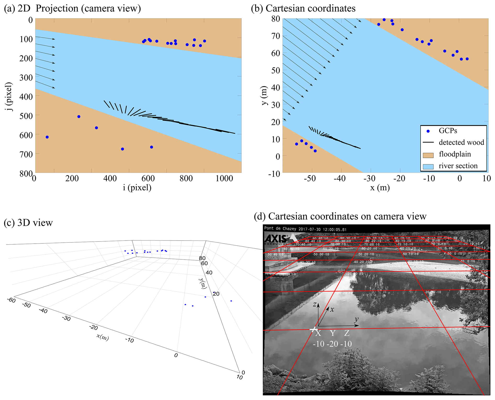
Figure 6Image rectification process. The non-colinear GCPs localization within the image (a) and the relative 2D metric coordinates for a given water level (b). The different solid lines represent the successive detection in a set of consecutive frames. (c) 3D view of non-colinear GCPs in metric coordinates. (d) Rectifying transformation matrix on the Ain River at a low flow level with the camera at (0,0,0).
The software was developed to provide a single environment for the analysis of wood pieces on the surface of the water from streamside videos. It consists of four distinct modules: detection, annotation, training, and performance. The home screen allows the operator to select any of these modules. From within a module, a menu bar on the left side of the interface allows operators to switch from one module to another. In the following sections, the operation of each of these modules is described.
4.1 Detection module
The detection module is the heart of the software. This module allows, from learned or manually specified parameters, the detecting of floating objects without human intervention (see Fig. 7). This module contains two main parts: (i) the detection tab, which allows the operator to open, analyze and export the results from one video or a set of videos; and (ii) the configuration tab, which allows the operator to load and save the software configuration by defining the parameters of wood detection (as described in Sect. 3), saving and extracting the results, and displaying the interface.
The detection process works as a video file player. The video file (or a stream URL) is loaded to let the software read the video until the end. When required, the reader generates a visual output, showing how the masks behave by adding color and information to the video content (see Fig. 7a). A small textual display area shows the frequency of past detections. Meanwhile, the software generates a series of files summarizing the positive outputs of the detection. They consist of YAML and CSV files, as well as image files to show the output of different masks and the original frames. A configuration tab is available and provides many parameters organized by various categories. The main configuration tab is divided into seven parts. The first part is dedicated to general configurations such as frames skipped between each computation and defining the areas within the frame where wood is not expected (e.g., bridge pier or riverbank). In the second and third parts, the parameters of the intensity and temporal masks are listed (see Sect. 3.1). The default values are μ=0.2 and σ=0.08 for the intensity mask and τ=0.25 and β=0.45 for the temporal mask. In the fourth and fifth parts, object tracking and characterization parameters are respectively defined as described in Sect. 3.2. Detection time is defined in the sixth part using an optical character recognition technique. Finally, the parameters of the orthorectification (see Sect. 3.3) are defined in the seventh part. The detection software can be used to process videos in batch (“script” tab), without generating a visual output, to save computing resources.
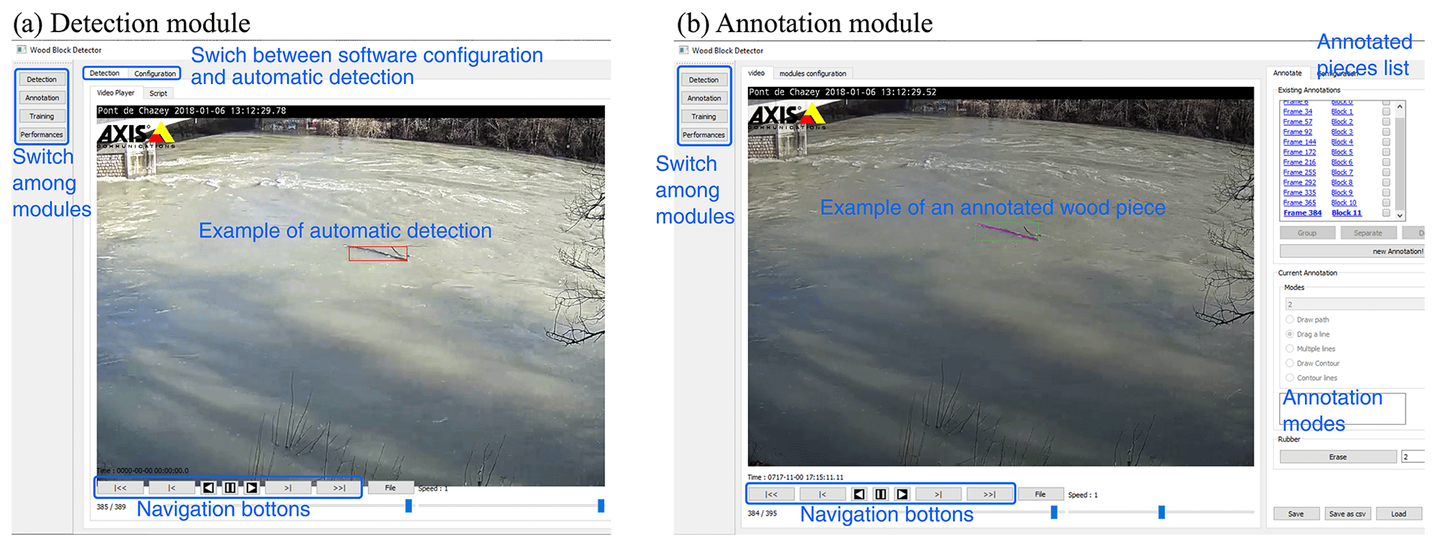
Figure 7User interface of (a) the detection module and (b) the annotation module of the automatic detection software.
4.2 Annotation module
As mentioned in Sect. 2, the detection procedure requires the classification of pixels and objects into wood and non-wood categories. To train and validate the automatic detection process, a ground truth or set of videos with manual annotations is required. Such annotations can be performed using different techniques. For example, objects can be identified with the help of a bounding box or selection of end points, as in MacVicar and Piégay (2012), Ghaffarian et al. (2020), and Zhang et al. (2021). It is also possible to sample wood pixels without specifying instances or objects and to sample pixels within annotated objects. Finally, objects and/or pixels can be annotated multiple times in a video sequence to increase the amount and detail of information in such an annotation database. This annotation process is time-consuming, so a trade-off must be made regarding the purpose of the annotated database and its required accuracy. Manual annotations are especially important when they are intended to be used within a training procedure, for which different lighting conditions, camera parameters, wood properties, and river hydraulics must be balanced. The rationale for manual annotations in the current study is presented in Sect. 5.1.
Given that the tool is meant to be as flexible as possible, the annotation module was developed to allow the operator to perform annotation in different ways depending on the purpose of the study. As shown in Fig. 7.b, this module contains three main parts: (i) the column on the far left allows the operator to switch to another module (detection, learning, or performance), (ii) the central part consists of a video player with a configuration tab for extracting the data, and (iii) the right part contains the tools to generate, create, visualize, and save annotations. The tools allow rather quick coarse annotation, similar to what was done by MacVicar and Piégay (2012) and Boivin et al. (2015), while still allowing the possibility of finer pixel-scale annotation. The principle of this module is to associate annotations with the frames of a given video. Annotating a piece of wood is like drawing its shape directly on a frame of the video using the drawing tools provided by the module. It is possible to add a text description to each annotation. Each annotation is linked to a single frame of the video; however, a frame can contain several annotations. An annotated video therefore consists of a video file and a collection of drawings, possibly with textual descriptions, associated with frames. It is possible to link annotations from one frame to another to signify that they belong to the same piece of wood. These data can be used to learn the movement of pieces of wood in the frame.
4.3 Performance module
The performance module allows the operator to set rules to compare automatic and manual wood detection results. This section also allows the operator to use a bare, pixel-based annotation or specify an orthorectification matrix to extract wood size metrics directly from the output of an automatic detection.
For this module an automatic detection file is first loaded, and then the result of this detection is compared with a manual annotation for that video if the latter is available. Comparison results are then saved in the form of a summary file (*.csv format), allowing the operator to perform statistical analysis of the results or the detection algorithm. A manual annotation file can only be loaded if it is associated with an automatic detection result.
The performance of the detected algorithm can be realized on several levels.
-
Object. The idea is to annotate one (or more) occurrence of a single object and to operate the comparison at bounding box scale. A detected object may comprehend a whole sequence of occurrences on several frames. It is validated when only a single occurrence happens to be related to an annotation. This is the minimum possible effort required to have an extensive overview of the object frequency on such an annotation database. This approach can, however, lead us to misjudge wrongly detected sequences as true positives (see below) or vice versa.
-
Occurrence. The idea is to annotate, even roughly, every occurrence of every woody object so that the comparison can happen between bounding boxes rather than at pixel level. Every occurrence of any detected object can be validated individually. This option requires substantially more annotation work than the object annotation.
-
Pixel. This case implies that every pixel of every occurrence of every object is annotated as wood. It is very powerful in evaluating algorithm performances and eventually refining its parameters with the help of some machine-learning technique. However, it requires extensive annotation work.
5.1 Assessment procedure
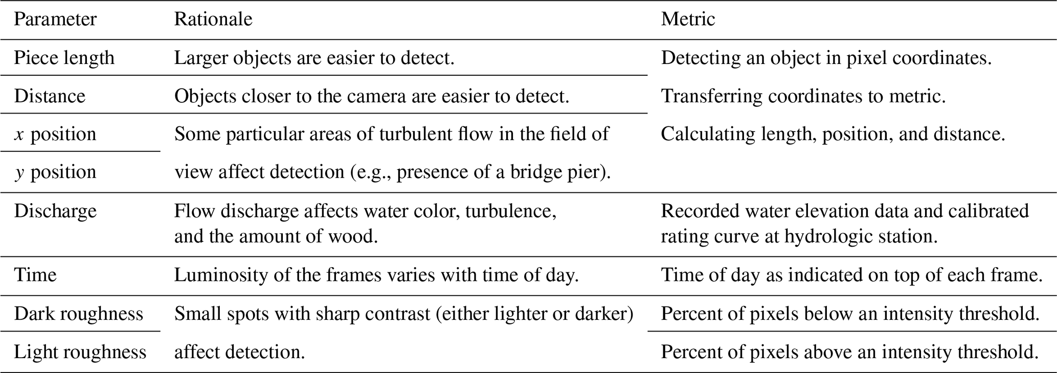
To assess the performance of the automatic detection algorithm, we used videos from the Ain River in France that were both comprehensively manually annotated and automatically analyzed. According to the data annotated by the observer, the performance of the software can be affected by different conditions: (i) wood piece length, (ii) distance from the camera, (iii, iv) wood x and y position, (v) flow discharge, (vi) daylight, and (vii, viii) light and darkness of the frame (see Table 2). If, for example, software detects a 1 cm piece at a distance of 100 m from the camera, there is a high probability that this is a false positive detection. Therefore, knowing the performance of the software in different conditions, it is possible to develop some rules to enhance the quality of data. The advantage of this approach is that all eight parameters introduced here are easily accessible in the detection process. In this section the monitoring details and annotation methods are introduced before the performance of the software is evaluated by comparing the manual annotations with the automatic detections.
Table 2Parameters used to assess the performance of the software.
Ghaffarian et al. (2020) and Zhang et al. (2021) show that the wood discharge (m3 per time interval) can be measured from the flux or frequency of wood objects (piece number per time interval). An object-level detection was thus sufficient for the larger goals of this research at the Ain River, which is to get a complete budget of transported wood volume.
A comparison of annotated with automatic object detections gives rise to three options.
-
True positive (TP). An object is correctly detected and is recorded in both the automatic and annotated database.
-
False positive (FP). An object is incorrectly detected and is recorded only in the automatic database.
-
False negative (FN). An object is not detected automatically and is only recorded in the annotated database.
Despite overlapping occurrences of wood objects in the two databases, the objects could vary in position and size between them. For the current study we set the TP threshold as the case in which either at least 50 % of the automatic and annotated bounding box areas were common or at least 90 % of an automatic bounding box area was part of its annotated counterpart.
In addition to the raw counts of TPs, FPs, and FNs, we defined two measures of the performances of the application, where
-
recall rate (RR) is the fraction of wood objects automatically detected (TP / (TP + FN)), and
-
precision rate (PR) is the fraction of detected objects that are wood (TP / (TP + FP)).
The higher the PR and the RR are, the more accurate our application is. However, both rates tend to interact. For example, it is possible to design an application that displays a very high RR (which means that it does not miss many objects) but suffers from a very low PR (it outputs a high amount of inaccurate data) and vice versa. Thus, we have to find a balance that is appropriate for each application.
It was well known from previous manual efforts to characterize wood pieces and develop automated detection tools that it is easier to detect certain wood objects than others. In general, the ability to detect wood objects in the dynamic background of a river in flood was found to vary with the size of the wood object, its position in the image frame, the flow discharge, the amount and variability of the light, interference from other moving objects such as spiders, and other weather conditions such as wind and rain. In this section, we describe and define the metrics that were used to understand the variability of the detection algorithm performance.
In general, more light results in better detection. The light condition can be changed by varying a set of factors such as weather conditions or the amount of sediment carried by the river. In any case, the daylight is a factor that can change the light condition systematically, i.e., low light early in the morning (Fig. 8a), bright light at midday with the potential for direct light and shadows (Fig. 8b), and low light again in the evening, though it is different from the morning because the hue is more bluish (Fig. 8c). This effect of the time of day was quantified simply by noting the time of the image, which was marked on the top of each frame of the recorded videos.
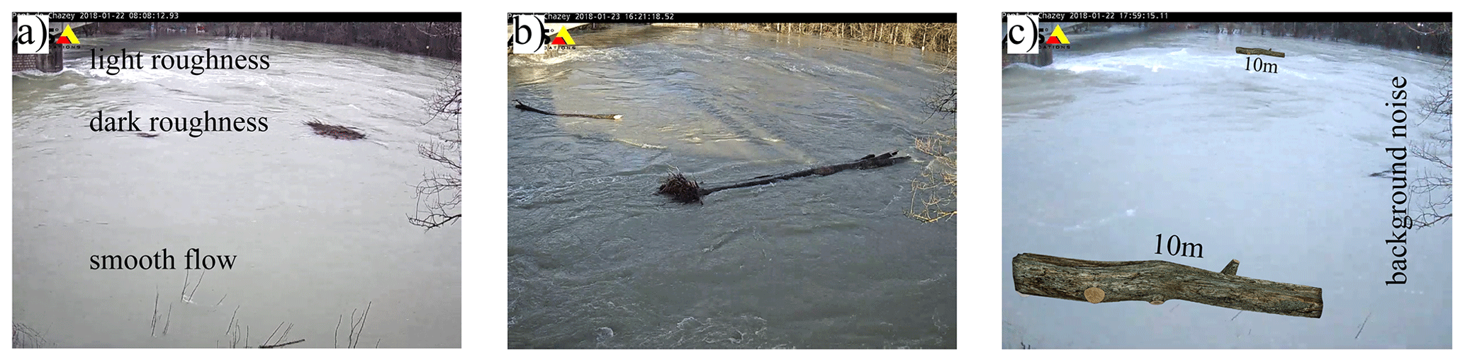
Figure 8Different light conditions during (a) morning, (b) noon, and (c) late afternoon result in different frame roughnesses and different detection performances. (c) Wood position can highly affect the quality of detection. Pieces that are passing in front of the camera are detected much better than the pieces far from the camera.
Detection is also strongly affected by the frame “roughness”, defined here as the variation in light over small distances in the frame. The change in light is important for the recognition of wood objects, but light roughness can also occur when there is a region with relatively light pixels due to something such as reflection of the surface of the water, and dark roughness can occur when there is a region with relatively dark pixels due to something such as shadows from the surface water waves or surrounding vegetation. Detecting wood is typically more difficult around light roughness, which results in false negatives, while the color map of a darker surface is often close to that of wood, which results in false positives. Both of these conditions can be seen in Fig. 8 (highlighted in Fig. 8a). In general, the frame roughness increases on windy days or when there is an obstacle in the flow, such as downstream of the bridge pier in the current case. The light roughness was calculated for the current study by defining a light intensity threshold and calculating the ratio of pixels of higher value among the frame. The dark roughness is calculated in the same way, but in this case the pixels less than the threshold were counted. In this work thresholds equal to 0.9 and 0.4 were used for light and dark roughness, respectively.
The oblique view of the camera means that the distance of the wood piece from the camera is another important factor in detection (Fig. 8c). The effect of distance on detection interacts with wood length; i.e., shorter pieces of wood that are not detectable near the camera may not be detectable toward the far bank due to the pixel size variation (Ghaffarian et al., 2020). Moreover, if a piece of wood passes through a region with high roughness (Fig. 8c) or amongst bushes or trees (Fig. 8c, right-hand side) it is more likely that the software is unable to detect it. In our case, 1 d of video record could not be analyzed due to the presence of a spider that moved around in front of the camera.
Flow discharge is another key variable in wood detection. Increasing flow discharge generally means that water levels are higher, which brings wood close to the near bank of the river closer to the camera. This change can make small pieces of wood more visible, but it also reduces the angle between the camera position and pixels, which makes wood farther from the camera harder to see. High flows also tend to increase surface waves and velocity, which can increase the roughness of the frame and lead to the wood being intermittently submerged or obscured. More suspended sediment is carried during high flows, which can change water surface color and increase the opacity of the water.
5.2 Detection performance
Automatic detection software performance was evaluated based on the event based TP, FP, and FN raw numbers as well as the precision (PR) and recall rates (RR) using the default parameters in the software. On average, manual annotation resulted in the detection of approximately twice as many wood pieces as the detection software (Table 3). Measured over all the events, RR = 29 %, which indicates that many wood objects were not detected by the software, while among detected objects about 36 % were false detections (PR =64 %).

To better understand model performance, we first tested the correlation between the factors identified in the previous section by calculating each of the eight parameters for all detections as one vector and then calculating the correlation between each pair of parameters (Table 4). As shown (the bold values), the pairs of dark–light roughness, length–distance, and discharge–time were highly correlated (correlations of 0.59, 0.46, and 0.37, respectively). For this reason, they were considered together to evaluate the performance of the algorithm within a given parameter space. The x/y positions were also considered as a pair despite a relatively low correlation (0.15) because they represent the position of an object. As a note, the correlation between time and dark roughness is higher than discharge and time, but we used the discharge–time pair because discharge has a good correlation only with time. As recommended by MacVicar and Piégay (2012), wood lengths were determined on a log-base-2 transformation to better compare different classes of floating wood, similar to what is done for sediment sizes.
Table 4Correlation between parameters. Values in bold show significant correlation.
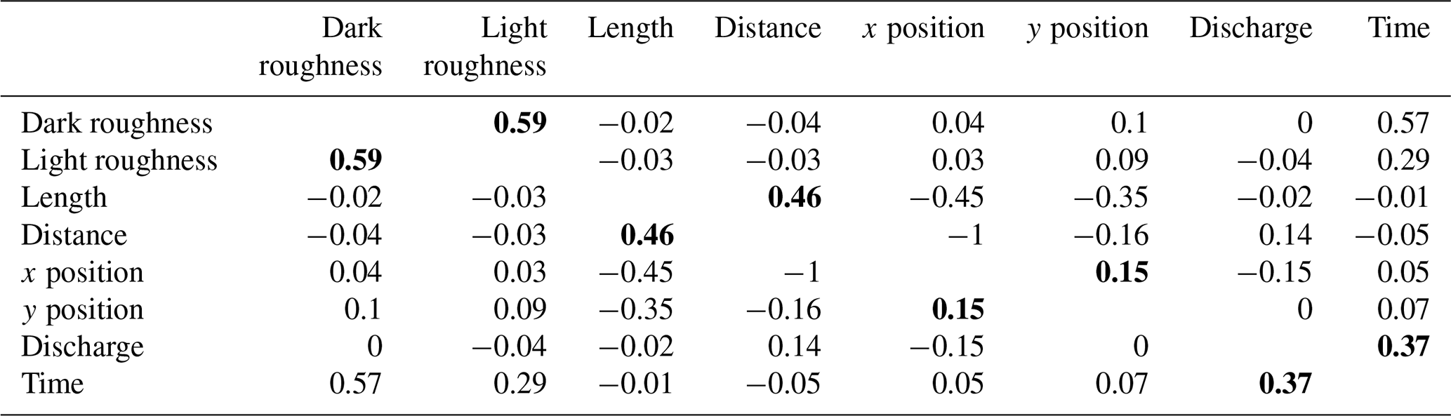
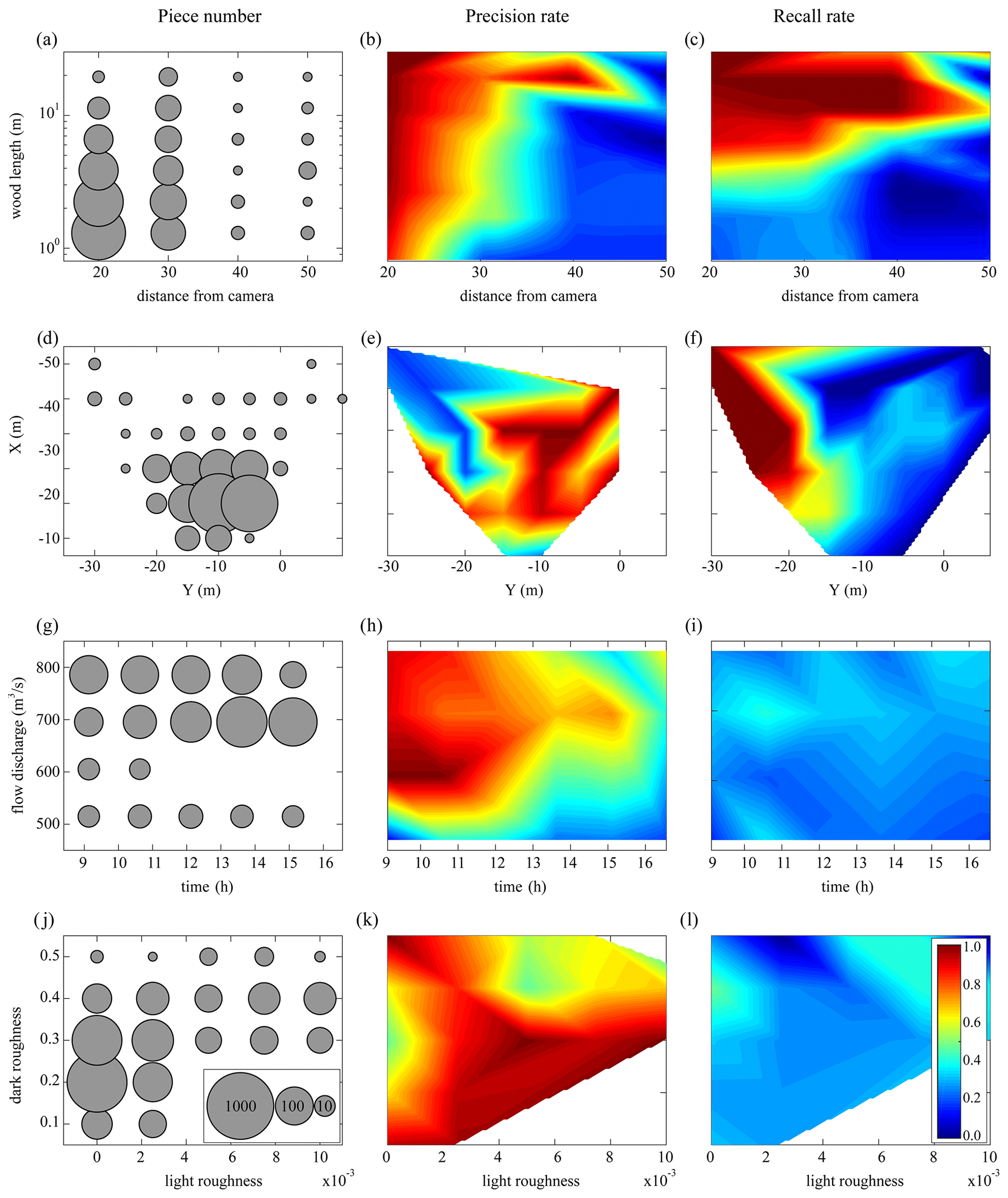
Figure 9Correction matrices: (a, b, c) wood lengths as a function of the distance from the camera, (d, e, f) detection position, (g, h, i) flow discharges during the daytime, and (j, k, l) light and dark roughnesses. The first column shows the number of all annotated pieces. The second and third columns show the precision and recall rates of the software, respectively.
The presentation of model performance by pairs of correlated parameters clarifies certain strengths and weaknesses of the software (Fig. 9). As expected, the results in Fig. 9b indicate that, first, the software is not so precise for small pieces of wood (less than the order of 1 m); second, there is an obvious link between wood length and the distance from the camera so that by increasing the distance from the camera, the software is precise only for larger pieces of wood. Based on Fig. 9e, the software precision is usually better on the right side of the frame than the left side. This spatial gradient in precision is likely because the software requires an object to be detected in at least 5 continuous frames for it to be recognized as a piece of wood (see Sect. 3.2 and Fig. 5 for more information), which means that most of the true positives are on the right side of the frame where five continuous frames have already been established. Also, the presence of the bridge pier (at X≅-30 to −40 m based on Fig. 9e) upstream produces lots of waves that decrease the precision of the software. Figure 9h shows that the software is much more precise during the morning when there is enough light rather than evening when the sunshine decreases. However, at low flow (Q<550 m3 s−1) the software precision decreases significantly. Finally, based on Fig. 9k, the software does not work well in two roughness conditions: (i) in a dark smooth flow (light roughness ≅0) when there are some dark patches (shadows) on the surface (dark roughness ≅0.3) and (ii) when roughness increases and there is a lot of noise in a frame (see Fig. 8).
To estimate the fraction of wood pieces that the software did not detect, the recall rate (RR) is calculated in different conditions, and a linear interpolation was applied to RR as presented in Fig. 9 (third column). According to Fig. 9c, RR is fully dependent on piece length so that for lengths of the order of 10 m (L=O(10)) RR is very good. By contrast, when L=O(0.1∼1), the RR is too small. There is a transient region when L=O(1), which slightly depends on the distance from the camera. One can say that the wood length is the most crucial parameter that affects the recall rate independent of the operator annotation. Based on Fig. 9f, the RR is much better on the left side of the frame than on the right side. It can be because the operator's eye needs some time to detect a piece of wood, so most of the annotations are on the right side of the frame. Having a small number of detections on the left side of the frame results in the small value of FN, which is followed by high values of RR in this region (RR=TP/(TP+FN). Therefore, while the position of detection plays a significant role in the recall rate, it is completely dependent on the operator bias. By contrast, frame roughness, daytime, and flow discharge do not play a significant role in the recall rate (Fig. 9i, l).
5.3 Post-processing
This section is separated into two main parts. First, we show how to improve the precision of the software by a posteriori distinction between TP and FP. After removing FPs from the detected pieces, in the second part, we test a process to predict the annotated data that the software missed, i.e., false negatives.
5.3.1 Precision improvement
To improve the precision of the automatic wood detection we first ran the software to detect pieces and extracted the eight key parameters for each piece as described in Sect. 5.1. Having the value of the eight key parameters (four pairs of parameters in Fig. 9) for each piece of wood, we then estimated the total precision of each object, as the average of four precisions from each panel in Fig. 9. In the current study the detected piece was considered to be a true positive if the total precision exceeded 50 %. To check the validity of this process, we used cross-validation by leaving one day out, calculating the precision matrices based on five other days, and applying the calculated PR matrices on the day that was left out. As is seen in Table 5, this post-processing step increases the precision of the software to 85 %, which is an enhancement of 21 %. The degree to which the precision is improved is dependent on the day left out for cross-validation. If, for example, the day left out had similar conditions as the mean, the PR matrices were well trained and were able to distinguish between TP and FP (e.g., 2 January with 42 % enhancement). On the other hand, if we have an event with new characteristics (e.g., very dark and cloudy weather or at discharges different from what we have in our database), the PR matrices were relatively blind and offered little improvement (e.g., 15 December with 10 % enhancement).
Table 5Precision rate (PR) before and after post-processing.
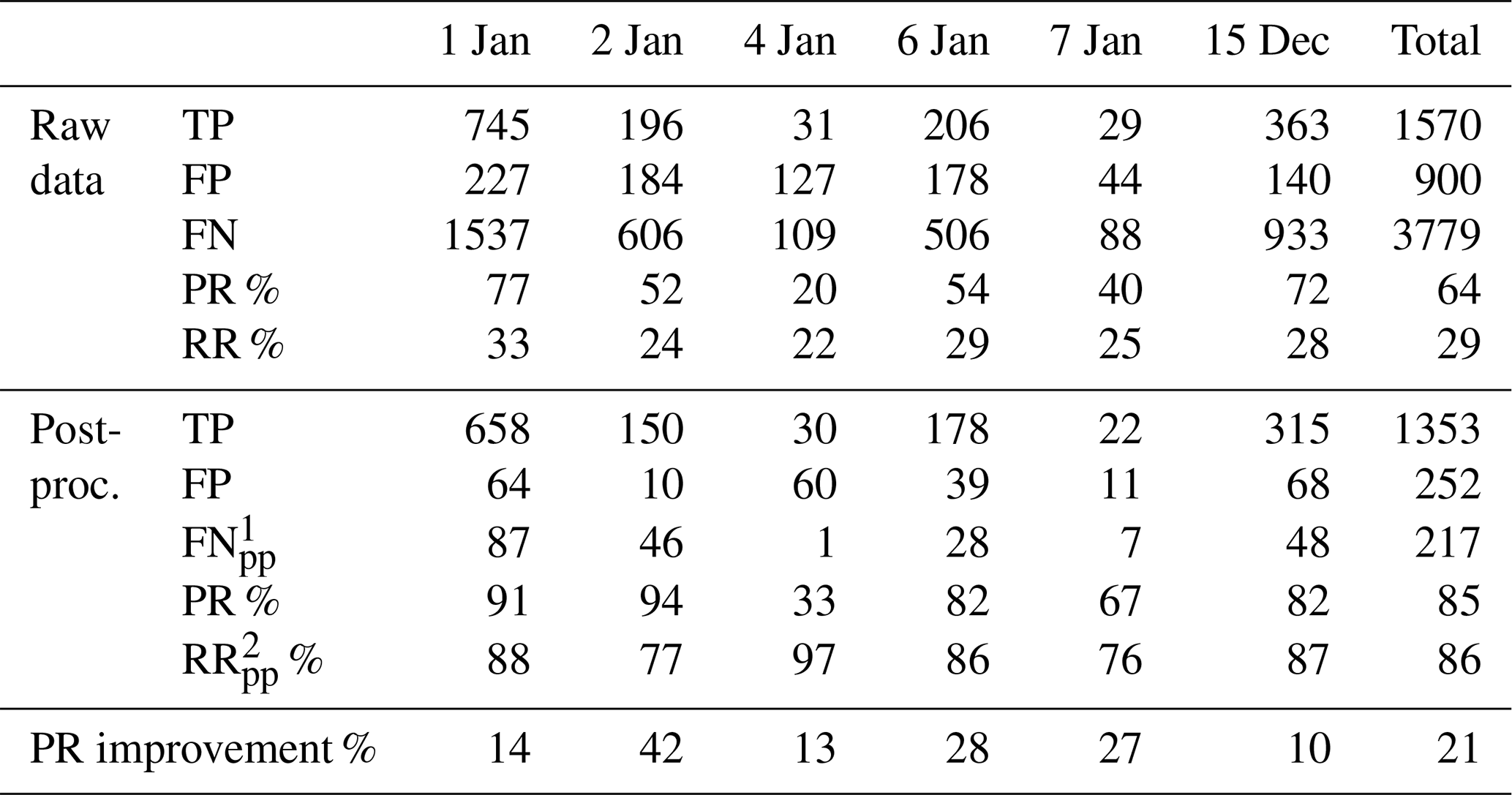
1FNpp denotes the false estimations of the precision matrices,
which results in missing some TP.
2RRpp denotes the recall rate of post-processing, which
corresponds to FNpp.
One difficulty with the post-processing reclassification of wood pieces is that this new step can also introduce error by classifying real objects as false positives (making them a false negative) or vice versa. Using the training data, we were able to quantify this error and categorize it as post-processed false negatives (FNpp) with an associated recall rate (RRpp). As shown in Table 5, the precision enhancement process lost only around 14 % of TPs (RRpp=86 %).
5.3.2 Estimating missed wood pieces based on the recall rate
The automated software detected 29 % of the manually annotated wood pieces (Table 5). In the previous section, methods were described that enhance the precision of the software by ensuring that these automatically detected pieces are TPs. The larger question, however, is how to estimate the missing pieces. Based on Fig. 9, both PR and RR are much higher for very large objects in most areas of the image and in most lighting conditions. However, the smaller pieces were found to be harder to detect, making the wood length the most important factor governing the recall rate. Based on this idea, the final step in post-processing is to estimate smaller wood pieces that were not detected by the software using the length distribution extracted by the annotations.
The estimation is based on the concept of a threshold piece length. Above the threshold, wood pieces are likely to be accurately counted using the automatic software. Below the threshold, on the other hand, the automatic detection software is likely to deviate from the manual counts. The length distribution obtained from the manual annotations (TP+FN) (Fig. 10a) was assumed to be the most realistic distribution that can be estimated from the video monitoring technique, and it was therefore used as the benchmark. Also shown are the raw results of the automatic detection software (TP+FP) and the raw results with the false positives removed (TP). At this stage, the difference between the TP and the TP+FN lines are the false negatives (FN) that the software has missed. Comparison between the two lines shows that they tend to deviate by 2–3 m. The correlation coefficient between the length distribution of TP as one vector and TP+FN as the other vector was calculated for thresholds varying from 1 cm to 15 m in length, and 2.5 m was defined as the optimum threshold length for recall estimation (Fig. 10b).
In the next step we wanted to estimate the pieces less than 2.5 m that the software missed. During the automatic detection process, when the software detects a piece of wood, according to Fig. 9 (third column), the RR can be calculated for this piece (same protocol as precision enhancement in Sect. 5.3.1). Therefore, if, for example, the average recall rate for a piece of wood is 50 %, there is likely to be another piece in the same condition (defined by the eight different parameters described in Table 2) that the software could not detect. To correct for these missed pieces, additional pieces were added to the database; note that these pieces were imaginary pieces inferred from the wood length distribution and were not detected by the software. Figure 10a shows the length distribution after adding these virtual pieces to the database (blue line, total of 5841 pieces). The result shows good agreement between this and the operator annotations (green line, total of 6249 pieces), which results in a relative error of only 6.5 % in the total number of wood pieces.
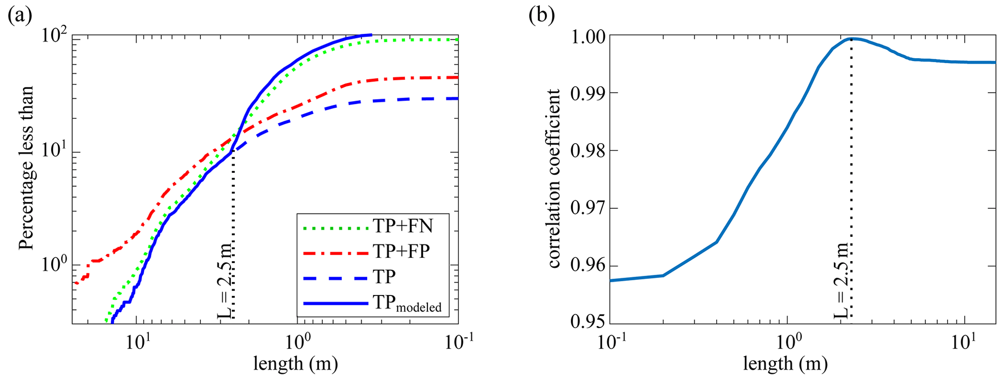
Figure 10(a) Steps to post-process software automatic detections: (i) raw detections (TP+FP, red line), (ii) only true positives using the PR improvement process (TP, blue dashed line), and (iii) modeling false negatives (blue line). Operator annotation (the green dotted line is used as a benchmark). (b) The correlation coefficient between operator annotation and modeled TP to find an optimum threshold length for RR improvement.
On the Ain River, by separating videos into 15 min segments, MacVicar and Piégay (2012) and Zhang et al. (2021) proposed the following equation for calculating wood discharge from the wood flux:
where Qw is the wood discharge (m3 per 15 min) and F is the wood flux (piece number per 15 min). Using this equation, the total volume of wood was calculated based on three different conditions: (i) operator annotation (TP+FN), (ii) raw data from the detection software (TP+FP), and (iii) post-processed data from the detection software (TPmodeled). Figure 11 shows a comparison of the total volume of wood from the manual annotations in comparison with the raw and post-processed annotations from the detection software. As shown, the raw detection results underestimate wood volume by almost 1 order of magnitude. After processing, the results show some scatter but are distributed around the 1:1 slope, which indicates that they follow the manual annotation results. There is a slight difference for days with lower fluxes (4 and 7 January), for which the post-processing tends to overestimate wood volumes, but in terms of an overall wood balance the volume of wood on these days is negligible. In total, 125 m3 of wood was annotated by the operator and the software automatically detected only 46 m3, some of which represent false positives. After post-processing, 142 m3 of wood was estimated to have passed in the analyzed videos for a total error of 13.5 %.
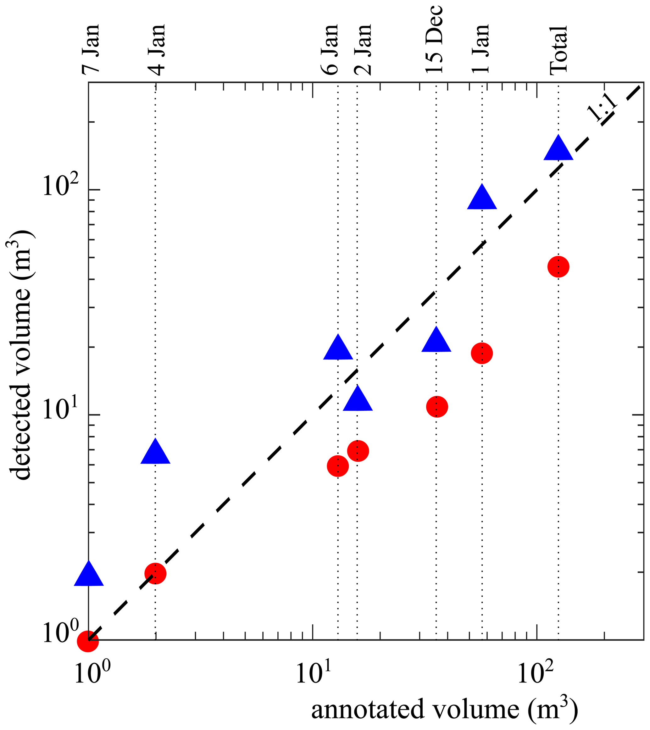
Figure 11Comparison of the total volume of wood between operator annotation as the benchmark and raw data (red circles) as well as post-processed data (blue triangles); compared with a 1:1 line.
Here, we present new software for the automatic detection of wood pieces on the river surface. After presenting the corresponding algorithm and the user interface, an example of automatic detection was presented. We annotated 6 d of flood events that were used to first check the performance of the software and then develop post-processing steps to remove possibly erroneous data and model data that were possibly missed by the software. To evaluate the performance of the software, we used precision and recall rates. The automatic detection software detects around one-third of all annotated wood pieces with a 64 % precision rate. Then, using the operator annotations as the ultimate goal, the post-processing part was applied to extrapolate data extracted from detection results, aiming to come as close as possible to the annotations. It is possible to detect false positives and increase the software precision to 86 % using four pairs of key factors: (i) light and dark roughness of the frame, (ii) daytime and flow discharge, (iii) x and y coordinates of the detection position, and (iv) distance of detection as a function of piece length. Using the concept of a threshold piece length for detection, it is then possible to model the missed wood pieces (false negatives). In the presented results, the final recall rate results in a relative error of only 6.5 % for piece number and 13.5 % for wood volume. It should be noted that the software cannot distinguish between a single piece of wood and pieces in a cluster of wood in congested wood fluxes.
This work shows the feasibility of the detection software to detect wood pieces automatically. Automation will significantly reduce the time and expertise required for manual annotation, making video monitoring a powerful tool for researchers and river managers to quantify the amount of wood in rivers. Therefore, the developed algorithm can be used to characterize wood pieces for a large image database at the study site. The results from the current study were all taken from a single site for which a large database of manual annotations was available to develop the correction procedures. In future applications it is unlikely that such a large database would be available. In such cases it is recommended to first ensure that the images collected are of high quality by following the recommendations in Ghaffarian et al. (2020) and Zhang et al. (2021). As data are collected, the automatic algorithm can be run to identify periods of high wood flux. Manual review of other high-water periods is also recommended to assess whether lighting conditions prevented the detection of wood. When suitable flood periods with floating wood are identified, manual annotations should be done to create the correction matrices. Future applications of this approach at a wide range of sites should lead to new insights on the variability of wood pieces at the reach and watershed scales in world rivers.
Finally, we think of this work as a first step towards more autonomous systems to detect and quantify wood in rivers. Applying the post-process steps in real time is a realistic next step because after we extract the correction matrices, which is a time-consuming process, the calculation time for PR and RR enhancement is negligible (less than 0.001 s per piece). Moreover, over recent years, automatic visual recognition tasks have progressed very with advances in machine-learning techniques, especially deep convolutional neural networks (DCNNs), that are now able to answer complex problems in real time. However, our context is very challenging for this class of solution since wood objects have a highly variable shape, and they are features in very noisy environments with a high variety of lighting conditions. Most training techniques are supervised, meaning that training an effective DCNN to solve this problem would require an extensive annotated dataset. The work presented in this paper can be used as a first step towards this solution. It can be used to help human operators quickly build an annotated dataset by correcting its output rather than annotating from scratch.
The database used in this study was a small part of a larger database that has been monitoring the Ain River since 2007. The entire database is undergoing editing and preparation and will be published soon.
HG was responsible for the application of statistical and computational techniques to analysis data, as well as the creation and presentation of the published work. HP, BM, and HG were responsible for the development and design of methodology and the creation of models. LT and PL worked on programming and software development. PL and ZZ performed the surveys and data collection. HP, BM, PL, and HG provided critical review, commentary, and revision. HP was responsible for oversight and leadership of the research activity planning and execution, including mentorship external to the core team.
The authors declare that they have no conflict of interest.
This work was performed within the framework and with the support of PEPS (RiskBof Project (2016)) and LABEX IMU (ANR-10-LABX-0088) and within the framework of EUR H2O'Lyon (ANR-17-EURE-0018) of Université de Lyon, with the latter two being part of the program “Investissements d'Avenir” (ANR-11-IDEX-0007) operated by the French National Research Agency (ANR).
This research has been supported by the LABEX IMU (grant no. ANR-10-LABX-0088), the EUR H2O'Lyon (grant no. ANR-17-EURE-0018), and the Université de Lyon (grant no. ANR-11-IDEX-0007).
This paper was edited by Giulia Sofia and reviewed by two anonymous referees.
Abbe, T. B. and Montgomery, D. R.: Patterns and processes of wood debris accumulation in the Queets river basin, Washington, Geomorphology, 51, 81–107, https://doi.org/10.1016/S0169-555X(02)00326-4, 2003.
Ali, I. and Tougne, L.: Unsupervised Video Analysis for Counting of Wood in River during Floods, in: Advances in Visual Computing, vol. 5876, edited by: Bebis, G., Boyle, R., Parvin, B., Koracin, D., Kuno, Y., Wang, J., Pajarola, R., Lindstrom, P., Hinkenjann, A., Encarnação, M. L., Silva, C. T., and Coming, D., Springer Berlin Heidelberg, Berlin, Heidelberg, 578–587, https://doi.org/10.1007/978-3-642-10520-3_55, 2009.
Ali, I., Mille, J., and Tougne, L.: Wood detection and tracking in videos of rivers, in: Scandinavian Conference on Image Analysis, 646–655, Berlin, https://doi.org/10.1007/978-3-642-21227-7_60, Heidelberg, 2011.
Ali, I., Mille, J., and Tougne, L.: Space–time spectral model for object detection in dynamic textured background, Pattern Recogn. Lett., 33, 1710–1716, https://doi.org/10.1016/j.patrec.2012.06.011, 2012.
Ali, I., Mille, J., and Tougne, L.: Adding a rigid motion model to foreground detection: application to moving object detection in rivers, Pattern Anal. Appl., 17, 567–585, https://doi.org/10.1007/s10044-013-0346-6, 2014.
Badoux, A., Andres, N., and Turowski, J. M.: Damage costs due to bedload transport processes in Switzerland, Nat. Hazards Earth Syst. Sci., 14, 279–294, https://doi.org/10.5194/nhess-14-279-2014, 2014.
Benacchio, V., Piégay, H., Buffin-Belanger, T., Vaudor, L., and Michel, K.: Automatioc imagery analysis to monitor wood flux in rivers (Rhône River, France), Third International Conference on Wood in World Rivers, available at: https://halshs.archives-ouvertes.fr/halshs-01618826 (last access: 2 June 2021), 2015.
Benacchio, V., Piégay, H., Buffin-Bélanger, T., and Vaudor, L.: A new methodology for monitoring wood fluxes in rivers using a ground camera: Potential and limits, Geomorphology, 279, 44–58, https://doi.org/10.1016/j.geomorph.2016.07.019, 2017.
Boivin, M., Buffin-Bélanger, T., and Piégay, H.: The raft of the Saint-Jean River, Gaspé (Québec, Canada): A dynamic feature trapping most of the wood transported from the catchment, Geomorphology, 231, 270–280, https://doi.org/10.1016/j.geomorph.2014.12.015, 2015.
Boivin, M., Buffin-Bélanger, T., and Piégay, H.: Interannual kinetics (2010–2013) of large wood in a river corridor exposed to a 50-year flood event and fluvial ice dynamics, Geomorphology, 279, 59–73, https://doi.org/10.1016/j.geomorph.2016.07.010, 2017.
Braudrick, C. A. and Grant, G. E.: When do logs move in rivers?, Water Resour. Res., 36, 571–583, https://doi.org/10.1029/1999WR900290, 2000.
Cerutti, G., Tougne, L., Vacavant, A., and Coquin, D.: A parametric active polygon for leaf segmentation and shape estimation, in: International symposium on visual computing, Las Vegas, United States, 202–213, 2011.
Cerutti, G., Tougne, L., Mille, J., Vacavant, A., and Coquin, D.: Understanding leaves in natural images–a model-based approach for tree species identification, Comput. Vis. Image Und. 117, 1482–1501, https://doi.org/10.1016/j.cviu.2013.07.003, 2013.
Comiti, F., Andreoli, A., Lenzi, M. A., and Mao, L.: Spatial density and characteristics of woody debris in five mountain rivers of the Dolomites (Italian Alps), Geomorphology, 78, 44–63, https://doi.org/10.1016/j.geomorph.2006.01.021, 2006.
ComputerVisionToolboxTM: The MathWorks, Inc., Natick, Massachusetts, United States., Release 2017b.
De Cicco, P. N., Paris, E., Ruiz-Villanueva, V., Solari, L., and Stoffel, M.: In-channel wood-related hazards at bridges: A review: In-channel wood-related hazards at bridges: A review, River Res. Applic., 34, 617–628, https://doi.org/10.1002/rra.3300, 2018.
Forsyth, D. and Ponce, J.: Computer vision: a modern approach, 2nd ed., Pearson, Boston, 1 pp., 2012.
Ghaffarian, H., Piégay, H., Lopez, D., Rivière, N., MacVicar, B., Antonio, A., and Mignot, E.: Video-monitoring of wood discharge: first inter-basin comparison and recommendations to install video cameras, Earth Surf. Proc. Land., 45, 2219–2234, https://doi.org/10.1002/esp.4875, 2020.
Gordo, A., Almazán, J., Revaud, J., and Larlus, D.: Deep Image Retrieval: Learning Global Representations for Image Search, in: Computer Vision – ECCV 2016, ECCV 2016, Lecture Notes in Computer Science, edited by: Leibe, B., Matas, J., Sebe, N., and Welling, M., vol 9910, Springer, Cham, https://doi.org/10.1007/978-3-319-46466-4_15, 2016.
Gregory, S., Boyer, K. L., and Gurnell, A. M.: Ecology and management of wood in world rivers, in: International Conference of Wood in World Rivers, 2000, Corvallis, Oregon, 2003.
Gurnell, A. M., Piégay, H., Swanson, F. J., and Gregory, S. V.: Large wood and fluvial processes, Freshwater Biol., 47, 601–619, https://doi.org/10.1046/j.1365-2427.2002.00916.x, 2002.
Haga, H., Kumagai, T., Otsuki, K., and Ogawa, S.: Transport and retention of coarse woody debris in mountain streams: An in situ field experiment of log transport and a field survey of coarse woody debris distribution: coarse woody debris in mountain streams, Water Resour. Res., 38, 1-1–1-16, https://doi.org/10.1029/2001WR001123, 2002.
Jacobson, P. J., Jacobson, K. M., Angermeier, P. L., and Cherry, D. S.: Transport, retention, and ecological significance of woody debris within a large ephemeral river, Water Resour. Res., 18, 429–444, 1999.
Keller, E. A. and Swanson, F. J.: Effects of large organic material on channel form and fluvial processes, Earth Surf. Process., 4, 361–380, https://doi.org/10.1002/esp.3290040406, 1979.
Kramer, N. and Wohl, E.: Estimating fluvial wood discharge using time-lapse photography with varying sampling intervals, Earth Surf. Proc. Land., 39, 844–852, 2014.
Kramer, N., Wohl, E., Hess-Homeier, B., and Leisz, S.: The pulse of driftwood export from a very large forested river basin over multiple time scales, Slave River, Canada, 53, 1928–1947, 2017.
Lassettre, N. S., Piégay, H., Dufour, S., and Rollet, A.-J.: Decadal changes in distribution and frequency of wood in a free meandering river, the Ain River, France, Earth Surf. Proc. Land., 33, 1098–1112, https://doi.org/10.1002/esp.1605, 2008.
Lejot, J., Delacourt, C., Piégay, H., Fournier, T., Trémélo, M.-L., and Allemand, P.: Very high spatial resolution imagery for channel bathymetry and topography from an unmanned mapping controlled platform, Earth Surf. Proc. Land., 32, 1705–1725, 2007.
Lemaire, P., Piegay, H., MacVicar, B., Mouquet-Noppe, C., and Tougne, L.: Automatically monitoring driftwood in large rivers: preliminary results, in: 2014 AGU Fall Meeting, San Francisco, 15–19 December 2014.
Lienkaemper, G. W. and Swanson, F. J.: Dynamics of large woody debris in streams in old-growth Douglas-fir forests, Can. J. Forest Res., 150–156, https://doi.org/10.1139/x87-02717, 1987.
Liu, L., Ouyang, W., Wang, X., Fieguth, P., Chen, J., Liu, X., and Pietikäinen, M.: Deep learning for generic object detection: A survey, Int. J. Comput. Vision, 128, 261–318, https://doi.org/10.1007/s11263-019-01247-4, 2020.
Lucía, A., Comiti, F., Borga, M., Cavalli, M., and Marchi, L.: Dynamics of large wood during a flash flood in two mountain catchments, Nat. Hazards Earth Syst. Sci., 15, 1741–1755, https://doi.org/10.5194/nhess-15-1741-2015, 2015.
Lyn, D., Cooper, T., and Yi, Y.-K.: Debris accumulation at bridge crossings: laboratory and field studies, Purdue University, West Lafayette, Indiana, https://doi.org/10.5703/1288284313171, 2003.
MacVicar, B. and Piégay, H.: Implementation and validation of video monitoring for wood budgeting in a wandering piedmont river, the Ain River (France), Earth Surf. Process. Landforms, 37, 1272–1289, https://doi.org/10.1002/esp.3240, 2012.
MacVicar, B. J., Piégay, H., Henderson, A., Comiti, F., Oberlin, C., and Pecorari, E.: Quantifying the temporal dynamics of wood in large rivers: field trials of wood surveying, dating, tracking, and monitoring techniques, Earth Surf. Process. Landforms, 34, 2031–2046, https://doi.org/10.1002/esp.1888, 2009a.
MacVicar, B. J., Piégay, H., Tougne, L., and Ali, I.: Video monitoring of wood transport in a free-meandering piedmont river, 2009, H54A-05, AGU, San Francisco, United States, 2009b.
Mao, L. and Comiti, F.: The effects of large wood elements during an extreme flood in a small tropical basin of Costa Rica, 67, 225–236, Debris Flow, Milan, Italy, https://doi.org/10.2495/DEB100191, 2010.
Marcus, W. A., Marston, R. A., Colvard Jr., C. R., and Gray, R. D.: Mapping the spatial and temporal distributions of woody debris in streams of the Greater Yellowstone Ecosystem, USA, Geomorphology, 44, 323–335, https://doi.org/10.1016/S0169-555X(01)00181-7, 2002.
Marcus, W. A., Legleiter, C. J., Aspinall, R. J., Boardman, J. W., and Crabtree, R. L.: High spatial resolution hyperspectral mapping of in-stream habitats, depths, and woody debris in mountain streams, Geomorphology, 55, 363–380, https://doi.org/10.1016/S0169-555X(03)00150-8, 2003.
Martin, D. J. and Benda, L. E.: Patterns of Instream Wood Recruitment and Transport at the Watershed Scale, T. Am. Fish. Soc., 130, 940–958, https://doi.org/10.1577/1548-8659(2001)130<0940:POIWRA>2.0.CO;2, 2001.
Mazzorana, B., Ruiz-Villanueva, V., Marchi, L., Cavalli, M., Gems, B., Gschnitzer, T., Mao, L., Iroumé, A., and Valdebenito, G.: Assessing and mitigating large wood-related hazards in mountain streams: recent approaches: Assessing and mitigating LW-related hazards in mountain streams, J. Flood Risk Manag., 11, 207–222, https://doi.org/10.1111/jfr3.12316, 2018.
Moulin, B. and Piegay, H.: Characteristics and temporal variability of large woody debris trapped in a reservoir on the River Rhone(Rhone): implications for river basin management, River Res. Applic., 20, 79–97, https://doi.org/10.1002/rra.724, 2004.
Muste, M., Fujita, I., and Hauet, A.: Large-scale particle image velocimetry for measurements in riverine environments, Water Resour. Res., 44, W00D19, https://doi.org/10.1029/2008WR006950, 2008.
Ravazzolo, D., Mao, L., Picco, L., and Lenzi, M. A.: Tracking log displacement during floods in the Tagliamento River using RFID and GPS tracker devices, Geomorphology, 228, 226–233, https://doi.org/10.1016/j.geomorph.2014.09.012, 2015.
Roussillon, T., Piégay, H., Sivignon, I., Tougne, L., and Lavigne, F.: Automatic computation of pebble roundness using digital imagery and discrete geometry, Comput. Geosci., 35, 1992–2000, https://doi.org/10.1016/j.cageo.2009.01.013, 2009.
Ruiz-Villanueva, V., Bodoque, J. M., Díez-Herrero, A., and Bladé, E.: Large wood transport as significant influence on flood risk in a mountain village, Nat. Hazards, 74, 967–987, https://doi.org/10.1007/s11069-014-1222-4, 2014.
Ruiz-Villanueva, V., Piégay, H., Gurnell, A. M., Marston, R. A., and Stoffel, M.: Recent advances quantifying the large wood dynamics in river basins: New methods and remaining challenges: Large Wood Dynamics, Rev. Geophys., 54, 611–652, https://doi.org/10.1002/2015RG000514, 2016.
Ruiz-Villanueva, V., Mazzorana, B., Bladé, E., Bürkli, L., Iribarren-Anacona, P., Mao, L., Nakamura, F., Ravazzolo, D., Rickenmann, D., Sanz-Ramos, M., Stoffel, M., and Wohl, E.: Characterization of wood-laden flows in rivers: wood-laden flows, Earth Surf. Process. Landforms, 44, 1694–1709, https://doi.org/10.1002/esp.4603, 2019.
Schenk, E. R., Moulin, B., Hupp, C. R., and Richter, J. M.: Large wood budget and transport dynamics on a large river using radio telemetry, Earth Surf. Process. Landforms, 39, 487–498, https://doi.org/10.1002/esp.3463, 2014.
Senter, A., Pasternack, G., Piégay, H., and Vaughan, M.: Wood export prediction at the watershed scale, Earth Surf. Proc. Land., 42, 2377–2392, https://doi.org/10.1002/esp.4190, 2017.
Senter, A. E. and Pasternack, G. B.: Large wood aids spawning Chinook salmon (Oncorhynchus tshawytscha) in marginal habitat on a regulated river in California, River Res. Appl., 27, 550–565, https://doi.org/10.1002/rra.1388, 2011.
Seo, J. I. and Nakamura, F.: Scale-dependent controls upon the fluvial export of large wood from river catchments, Earth Surf. Proc. Land., 34, 786–800, https://doi.org/10.1002/esp.1765, 2009.
Seo, J. I., Nakamura, F., Nakano, D., Ichiyanagi, H., and Chun, K. W.: Factors controlling the fluvial export of large woody debris, and its contribution to organic carbon budgets at watershed scales, Water Resour. Res., 44, https://doi.org/10.1029/2007WR006453, 2008.
Seo, J. I., Nakamura, F., and Chun, K. W.: Dynamics of large wood at the watershed scale: a perspective on current research limits and future directions, Landsc. Ecol. Eng., 6, 271–287, https://doi.org/10.1007/s11355-010-0106-3, 2010.
Turowski, J. M., Badoux, A., Bunte, K., Rickli, C., Federspiel, N., and Jochner, M.: The mass distribution of coarse particulate organic matter exported from an Alpine headwater stream, Earth Surf. Dynam., 1, 1–11, https://doi.org/10.5194/esurf-1-1-2013, 2013.
Viola, P. A. and Jones, M. J.: Object recognition system, J. Acoust. Soc. Am., https://doi.org/10.1121/1.382198, 2006.
Warren, D. R. and Kraft, C. E.: Dynamics of large wood in an eastern US mountain stream, Forest Ecol. Manage., 256, 808–814, https://doi.org/10.1016/j.foreco.2008.05.038, 2008.
Wohl, E.: Floodplains and wood, Earth Sci. Rev., 123, 194–212, https://doi.org/10.1016/j.earscirev.2013.04.009, 2013.
Wohl, E. and Scott, D. N.: Wood and sediment storage and dynamics in river corridors, Earth Surf. Proc. Land., 42, 5–23, https://doi.org/10.1002/esp.3909, 2017.
Zevenbergen, L. W., Lagasse, P. F., Clopper, P. E., and Spitz, W. J.: Effects of Debris on Bridge Pier Scour, in: Proceedings 3rd International Conference on Scour and Erosion (ICSE-3), 1–3 November 2006, Amsterdam, The Netherlands, Gouda (NL): CURNET. S., 741–749, 2006.
Zhang, Z., Ghaffarian, H., MacVicar, B., Vaudor, L., Antonio, A., Michel, K., and Piégay, H.: Video monitoring of in-channel wood: From flux characterization and prediction to recommendations to equip stations, Earth Surf. Proc. Land., 46, 822–836, https://doi.org/10.1002/esp.5068, 2021.