


Impact Statement
A deep understanding of bacterial morphology and behaviour is crucial to minimize undesirable and maximize beneficial effects of microorganisms on human health and welfare. Interestingly, functionalities and mechanisms of some microrobots with promising biomedical applications are motivated by flagellated bacteria; therefore, investigating influences of different types of flagella (puller/pusher) and their arrangement on the microrobots’ locomotion paves the way to optimize and enhance the performance of the robots. By simulating the locomotion of a bi-flagellated bacterium in Newtonian viscous fluid, we show that, depending on the flagellum arrangement, a bacterium morphologically like Magnetococcus marinus (MC-1) moves on a double helical trajectory with different sizes. This outcome is consistent with some experimental observation of MC-1 locomotion. Moreover, we quantitatively demonstrate the importance of a puller flagellum in the bacterial locomotion and examine the effect of an overwhirling pusher flagellum on swimming of a bi-flagellated model bacterium.
1. Introduction
The locomotion of microorganisms, such as bacteria, has been a topic of a lot of research and mathematical analysis in recent decades (Reference HigdonHigdon, 1979; Reference Shum and GaffneyShum & Gaffney, 2015b; Reference TaylorTaylor, 1951). Bacteria play a vital role in the ecosystem and have a lot of applications in human life, from medicine to industry and agriculture (Reference AmargerAmarger, 2002; Reference Felfoul, Mohammadi, Taherkhani, De Lanauze, Xu, Loghin and MartelFelfoul et al., 2016; Reference Sengun and KarabiyikliSengun & Karabiyikli, 2011). Some kinds of bacteria swim though a fluid by rotating flexible flagella to generate a propulsive force. The swimming mechanisms vary among the species; some species, such as Escherichia coli, form a flagellar bundle (Reference Flores, Lobaton, Méndez-Diez, Tlupova and CortezFlores, Lobaton, Méndez-Diez, Tlupova, & Cortez, 2005), whereas others, such as Vibrio alginolyticus, are propelled by a single flagellum. These differences in morphology give rise to different patterns of motility and reorientation, including run-and-tumble (Reference BergBerg, 1975) and forward–reverse flick (Reference Jabbarzadeh and FuJabbarzadeh & Fu, 2018; Reference Xie, Altindal, Chattopadhyay and WuXie, Altindal, Chattopadhyay, & Wu, 2011).
In addition to the interest in fundamental knowledge about the morphology of bacteria and their interaction with the environment, interest in using bacteria or fabricating bacterium-mimicking microrobots has grown in recent years (Reference Felfoul, Mohammadi, Taherkhani, De Lanauze, Xu, Loghin and MartelFelfoul et al., 2016; Reference Li, de Ávila, Gao, Zhang and WangLi, de Ávila, Gao, Zhang, & Wang, 2017). In this regard, magnetotactic bacteria (MTB) are of particular interest since they can be steered by applying an external magnetic field. Among the magnetotactic bacteria, Magnetococcus marinus (MC-1) is commonly studied and its biomedical applications for drug delivery have already been examined (Reference Felfoul, Mohammadi, Taherkhani, De Lanauze, Xu, Loghin and MartelFelfoul et al., 2016). However, these applications are not limited to MTB; naturally, non-magnetic microorganisms can also be directed by magnetic field after incorporation of magnetic particles (Reference Park, Zhuang, Yasa and SittiPark, Zhuang, Yasa, & Sitti, 2017).
One of the striking differences between the MC-1 and widely studied bacteria, such as E. coli, is that MC-1 has two sheathed bundles of flagella on one side of the cell body. Each bundle is composed of seven flagellar filaments and many fibrils enveloped in a sheath. This structure of two bundles allows the bacteria to swim at speeds of up to  $500\,{\mathrm {\mu }}{\rm m}\,{\rm s}^{-1}$ (Reference Bente, Mohammadinejad, Charsooghi, Bachmann, Codutti, Lefèvre, Klumpp and FaivreBente et al., 2020). Magnetosomes, intracellular structures containing iron sulphide or iron oxide nano-particles, allow MC-1 to navigate by the Earth's magnetic field (Reference Mohammadinejad, Faivre and KlumppMohammadinejad, Faivre, & Klumpp, 2021).
Whereas the locomotion of uni-flagellated bacteria has been well studied and, in many cases, a uni-flagellated model adequately reproduces behaviour in experiments even with multi-flagellated bacteria (Reference Park, Kim and LimPark, Kim, & Lim, 2019a, Reference Park, Kim and Lim2019b; Reference Shum and GaffneyShum & Gaffney, 2015a; Reference Tokárová, Perumal, Nayak, Shum, Kašpar, Rajendran and NicolauTokárová et al., 2021), more specialized models are required to understand bundling, wrapping and other complex phenomena with multiple flagella (Reference Constantino, Jabbarzadeh, Fu, Shen, Fox, Haesebrouck, Linden and BansilConstantino et al., 2018; Reference Flores, Lobaton, Méndez-Diez, Tlupova and CortezFlores et al., 2005; Reference Nguyen and GrahamNguyen & Graham, 2018). The unusual morphology and swimming style of MC-1 warrants further study. In earlier theoretical studies of MC-1, it was assumed that the two flagellar bundles are behind the cell body and their synchronous rotations push the cell forward. Based on this assumption, the model bacterium swims in a relatively straight trajectory in the absence of a magnetic field; it exhibits helical motion when a magnetic field is applied (Reference ShumShum, 2019; Reference Yang, Chen, Ma, Wu and SongYang, Chen, Ma, Wu, & Song, 2012). These results are inconsistent with some experimental observations (Reference Bente, Mohammadinejad, Charsooghi, Bachmann, Codutti, Lefèvre, Klumpp and FaivreBente et al., 2020), indicating that MC-1 travels along a double helical trajectory in the absence of magnetic field effects. Numerical simulations based on the Stokesian dynamics simulation method showed that such a double helical trajectory can be produced if one of the flagellar bundles pushes the cell while the other pulls.
Reference Yang, Chen, Ma, Wu and SongYang et al. (2012) numerically and experimentally studied the effects of an external magnetic field on the locomotion of MC-1. In their model, two rigid helical flagella push forward a prolate spheroidal cell body containing a magnetosome chain in a specific alignment. They employed resistive force theory to model the hydrodynamic interactions and showed that there is a good agreement between the numerical and experimental results as they apply a wide range of magnetic fields for different inclinations of magnetic moment.
Reference ShumShum (2019) used a boundary element method (BEM) to simulate the motion of a model bacterium with two rigid pusher flagella near a surface. He found that placing the two flagella far apart reduces the cell body rotation rate. This could help the bacterium to move faster and achieve a better alignment with an external magnetic field. In addition, he showed that position and orientation of the flagella are two main factors which determine the bacterium behaviour in remaining trapped at a solid surface or escaping back to the bulk fluid.
Reference Mohammadinejad, Faivre and KlumppMohammadinejad et al. (2021) developed a model based on Stokesian dynamics and Kirchhoff's rod model to investigate the locomotion of a MTB with a flexible pusher flagellum and spherical cell body in the presence of an external magnetic field. They focused on the response of MTB to reversal of the external magnetic field and found that the diameter of the U-turn and the turning time are smaller for stronger magnetic fields. Moreover, they noted that the model bacterium undergoes a double helical motion when, simultaneously, the magnetic field is strong and the angle between the flagellum axis and the magnetic moment is large enough.
Several studies have specifically focused on motions of a rotating elastic filament in a viscous fluid to understand the dynamics of bacterial flagellar hooks and filaments (Reference Jabbarzadeh and FuJabbarzadeh & Fu, 2020; Reference Lee, Kim, Olson and LimLee, Kim, Olson, & Lim, 2014; Reference Lim and PeskinLim & Peskin, 2004; Reference Wolgemuth, Powers and GoldsteinWolgemuth, Powers, & Goldstein, 2000). In one of the recent studies, Reference Park, Kim, Ko and LimPark, Kim, Ko, and Lim (2017) showed that a rotating flexible helical filament exhibits three regimes of dynamical motion: twirling and overwhirling motions which are stable and an unstable whirling motion. The type of motion that emerges depends on the physical parameters of the fluid, the rotation frequency and the elastic properties of the filament. At a constant rotation frequency, if the stiffness of a helical filament is above a critical value then the filament rotates about its straight rotation axis; this is called stable twirling motion. If the stiffness is below a critical value then twirling becomes unstable and motion transitions to stable overwhirling, which is characterized by a curved axis such that the free end of the filament is close to the driven end. Between the twirling and overwhirling regimes, the filament exhibits unstable whirling motion, in which the axis of the filament is slightly curved and rotates about the motor axis.
In the present work, we first develop an elastohydrodynamic model to study the locomotion of a bi-flagellated bacterium with one puller and one pusher flexible flagellum. The pusher and puller flagella are both right-handed helices but rotate in the clockwise (CW) and counterclockwise (CCW) directions, respectively (viewed with the flagellum between the cell body and the observer), and hence apply ‘pushing’ and ‘pulling’ forces, respectively, on the cell body. Generally, the bacterium then swims with the pusher flagellum at the rear of the cell body and the puller flagellum in front of the body. Such a morphology is inspired by the observations of Reference Bente, Mohammadinejad, Charsooghi, Bachmann, Codutti, Lefèvre, Klumpp and FaivreBente et al. (2020), in which they concluded that MC-1 most likely swims with one puller and one pusher flagellar bundle. Here, we use a regularized Stokes formulation (Reference Olson, Lim and CortezOlson, Lim, & Cortez, 2013) in conjunction with a BEM (Reference PozrikidisPozrikidis, 2002) to model the hydrodynamic interactions of the model bacterium components. We assume that the two flexible filaments, which represent the two flagellar bundles in MC-1, are inextensible and unshearable and only allowed to bend and twist, following a discretization of the Kirchhoff rod model (Reference Lim, Ferent, Wang and PeskinLim, Ferent, Wang, & Peskin, 2008). Since each bundle of flagella is modelled by a single flexible filament, wherever we refer to a flagellum or flexible filament in our results, it should be interpreted as a sheathed flagellar bundle in MC-1. In the next step, the proposed model is validated and the swimming styles of three model bacteria (pusher, pusher–pusher, puller–pusher) are compared. Finally, the influence of various parameters including the flagellar stiffness, position, orientation and the ratio of the two motors’ torques on swimming characteristics of puller–pusher bacterium is studied in more detail.
2. Modelling and methods
2.1 Geometric model
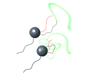
The model bacterium consists of one rigid spherical cell body, one puller flagellum (dark slate grey) and one pusher flagellum (grey), as shown in figure 1. The cell body has centroid position denoted by  $\boldsymbol {X}^{(B)}$ and orientation described by the basis
  $\{\boldsymbol {e}_1^{(B)},\boldsymbol {e}_2^{(B)},\boldsymbol {e}_3^{(B)}\}$. The pusher flagellum has position
  $\boldsymbol {X}^{(1)}$ and basis
  $\{\boldsymbol {e}_1^{(1)},\boldsymbol {e}_2^{(1)},\boldsymbol {e}_3^{(1)}\}$, and the puller flagellum has position
  $\boldsymbol {X}^{(2)}$ and basis
  $\{\boldsymbol {e}_1^{(2)},\boldsymbol {e}_2^{(2)},\boldsymbol {e}_3^{(2)}\}$. All of the aforementioned bases are right-handed and orthonormal. In this study, it is assumed that the two flagella have identical physical and elastic properties and their initial and rest configurations are right-handed helices with centrelines given by
 \begin{equation} \boldsymbol{\varLambda}^{(i)}(\xi) = \boldsymbol{X}^{(i)} + \xi\boldsymbol{e}_1^{(i)} + \varXi(\xi) \cos{(2{\rm \pi}\xi/p)}\boldsymbol{e}_2^{(i)} + \varXi(\xi)\sin{(2{\rm \pi}\xi/p)}\boldsymbol{e}_3^{(i)},\end{equation}
where  $i=1,2$ for the pusher and the puller flagella, respectively; the variable
  $\xi$ parameterizes the distance along the axis of the helix with
  $0\leqslant \xi \leqslant L_F$,
  $\varXi (\xi )=a(1-\exp ({-(k_E\xi )^2}))$ is the helix amplitude function and
  $a$,
$a$,  $p$ and
  $k_E$ represent the maximum helix amplitude, the helix pitch and the amplitude growth rate (the amplitude grows from zero to
  $a$ over a region of length roughly
  ${2}/{k_E}$), respectively. The position and orientation of the puller flagellum is specified by two angles
  $\alpha$ and
  $\beta$ defined on the
  $\boldsymbol {e}_1^{(B)}$–
 $\boldsymbol {e}_3^{(B)}$ plane through the centre of the cell body. The pusher flagellum is placed symmetrically on the other side of the cell body with the same acute angles as the puller flagellum (figure 1). In all simulations, except one set of simulations where we specifically study the influence of the angle
  $\beta$, we assume that the rotors are normal to the cell membrane (i.e.
  $\beta =\alpha$). In studying the influence of
  $\beta$, the angle
  $\alpha$ is constant and
  $|\alpha -\beta |$ represents how much the rotors deviate from being normal to the cell membrane.

Figure 1. A schematic view of the model bacterium in which different bases and vectors are used to describe the position and orientation of the components. Here, the  $\alpha$ and
  $\beta$ angles represent the position and orientation of the rotors on the cell body, defined with respect to
  $\boldsymbol {e}_1^{(B)}$. The internal moment between the
  $n$th and
  $(n+1)$th segments is denoted by
  $\boldsymbol {N}^{(i)n+{1}/{2}}$. Note that the thickness of the flagella in the figures does not reflect the actual thickness of the flagella in the model bacterium.
The experimental observations have shown that the cell body of MC-1 is approximately spherical (Reference Bente, Mohammadinejad, Charsooghi, Bachmann, Codutti, Lefèvre, Klumpp and FaivreBente et al., 2020; Reference Tokárová, Perumal, Nayak, Shum, Kašpar, Rajendran and NicolauTokárová et al., 2021). Based on the measurements for MC-1, the cell body diameter is  $1.3\pm 0.1\,\mathrm {\mu }$m and the flagellum length is
  $3.3\pm 0.4\,\mathrm {\mu }$m (Reference Bente, Mohammadinejad, Charsooghi, Bachmann, Codutti, Lefèvre, Klumpp and FaivreBente et al., 2020). We are unaware of any study that measures the flexibility of the flagella or flagellar bundles in MC-1. Recalling that a filament in our model represents multiple flagella in a bundle, we use values of the rigidity approximately 1.5–11 times that of a flagellum in E. coli (
 $3.5\,{\rm pN}\,{\mathrm {\mu }}{\rm m}^2$ Reference Darnton and BergDarnton & Berg, 2007). Other parameters in this study, such as the motors’ torques, helical pitch and amplitude are chosen from the values given by Reference Bente, Mohammadinejad, Charsooghi, Bachmann, Codutti, Lefèvre, Klumpp and FaivreBente et al. (2020), Reference Mohammadinejad, Faivre and KlumppMohammadinejad et al. (2021) and Reference ShumShum (2019). Here, these parameters are non-dimensionalized by the averaged cell body radius
  $0.65\,\mathrm {\mu }$m (Reference Bente, Mohammadinejad, Charsooghi, Bachmann, Codutti, Lefèvre, Klumpp and FaivreBente et al., 2020), MC-1's motor torque which is approximately
  $12\,{\rm pN}\,\mathrm {\mu }$m (Reference Bente, Mohammadinejad, Charsooghi, Bachmann, Codutti, Lefèvre, Klumpp and FaivreBente et al., 2020) and the swimming fluid viscosity
  $\mu =10^{-3}$ Pa s.
2.2 Hydrodynamic interactions
In modelling of bacterial locomotion, the Reynolds number is very small and so the hydrodynamic interactions are governed by the incompressible Stokes equations
 \begin{equation} {-}\boldsymbol{\nabla} p + \mu \Delta \boldsymbol{u} + \boldsymbol{F_b} = \boldsymbol{0},\quad \boldsymbol{\nabla} \boldsymbol{\cdot} \boldsymbol{u} = 0,\end{equation}
where  $\mu$ is the fluid viscosity,
  $p$ is the fluid pressure,
  $\boldsymbol {u}$ is the fluid velocity and
  $\boldsymbol {F_b}$ is the force per unit volume applied to the fluid by the immersed body. The model bacterium exerts a distribution of viscous stress
  $\boldsymbol {f}_{head}$ over the surface
  $S$ of the cell body (three-dimensional spherical cell body) and distributions of the viscous stress
  $\boldsymbol {f}_{fla}$ and viscous torque
  $\boldsymbol {n}$ along the centrelines of the flagella
  $\varGamma ^{(i)}$. We use the superscript
  $(i)$ to distinguish the pusher flagellum
  $(i=1)$ from the puller one
  $(i=2)$. Since both flagella are right-handed, the rotors in the pusher and puller flagella rotate in
  $-\boldsymbol {e}_1^{(1)}$ and
  $\boldsymbol {e}_1^{(2)}$ directions, respectively, to provide propulsion. In a Lagrangian description, the elastic filaments
  $\varGamma ^{(i)}$, which rotate and deform in time, and the cell body
  $S$ can be represented by a three-dimensional space curve
  $\boldsymbol {\gamma }(s,t)$ and surface
  $\,\boldsymbol {\varPsi }(\theta,\phi,t)$, respectively. The variables
  $s$,
$s$,  $\theta$ and
  $\phi$ are material coordinates along the filament (initialized as arclength) and the cell body surface, respectively, and
  $t$ is time. To ease the presentation, we let the variables
  $\boldsymbol {f}_{fla}(s,t)$,
  $\boldsymbol {n}(s,t)$ and
  $\boldsymbol {\gamma }(s,t)$ denote the respective quantities for both flagella with the understanding that the integral over
  $\varGamma ^{(i)}\ (i=1,2)$ involves the variables associated with the respective flagellum. The body force can be written as
 \begin{align} \boldsymbol{F_b}(\boldsymbol{x},t)& = \oint_{S} {\boldsymbol{f}_{head}(\theta,\phi,t) \delta(\boldsymbol{x}-\boldsymbol{\varPsi}(\theta,\phi,t))\,{\rm d} A} + \sum_{i = 1}^{2}{\int_{\varGamma^{(i)}} {\boldsymbol{f}_{fla}(s,t)\delta(\boldsymbol{x}-\boldsymbol{\gamma}(s,t))\,{\rm d} s}} \nonumber\\ &\quad + \sum_{i = 1}^{2}{\frac{1}{2}\boldsymbol{\nabla}\times\int_{\varGamma^{(i)}} {\boldsymbol{n}(s,t)\delta(\boldsymbol{x}-\boldsymbol{\gamma}(s,t))\,{\rm d} s}}. \end{align}
The evaluation point  $\boldsymbol {x}$ can be anywhere in
  $\mathbb {R}^3$ including the model bacterium surface. To represent the flagellum thickness and avoid the singularity and also to enhance the stability of the solution, we use a regularized Stokes formulation for the flagella. Therefore, we replace the delta function (
 $\delta$) by a cutoff function
  $\psi _\epsilon$ in the second and third integrals. The radially symmetric cutoff function approximates the delta function in three dimensions. Following previous studies using the method of regularized stokeslets (Reference Cortez, Fauci and MedovikovCortez, Fauci, & Medovikov, 2005; Reference Olson, Lim and CortezOlson et al., 2013), we choose the cutoff function as
 \begin{equation} \psi_\epsilon(\boldsymbol{x}) = \frac{15\epsilon^4}{8{\rm \pi} ({\Vert \boldsymbol{x} \Vert}^2 + \epsilon^2)^{7/2}},\end{equation}
where we assume that  $\epsilon ={d}/{2}$ to represent the filament radius. The solution for the flow field satisfying (2.2a,b) and (2.3) can be written as the boundary integral equations (Reference Cortez, Fauci and MedovikovCortez et al., 2005; Reference Olson, Lim and CortezOlson et al., 2013)
 \begin{align} \boldsymbol{u}(\boldsymbol{x},t)& = \oint_{S}{\boldsymbol{f}_{head}J_3 + [\,\boldsymbol{f}_{head}\boldsymbol{\cdot} (\boldsymbol{x}-\boldsymbol{\varPsi})](\boldsymbol{x}-\boldsymbol{\varPsi})J_4\,{\rm d} A} + \sum_{i = 1}^{2}{\int_{\varGamma^{(i)}}{\boldsymbol{f}_{fla}J_1 + [\,\boldsymbol{f}_{fla}\boldsymbol{\cdot} (\boldsymbol{x}-\boldsymbol{\gamma})](\boldsymbol{x}-\boldsymbol{\gamma})J_2\,{\rm d} s}} \nonumber\\ &\quad + \sum_{i = 1}^{2}{\frac{1}{2}\boldsymbol{\nabla}\times\int_{\varGamma^{(i)}}{[\boldsymbol{n} \times(\boldsymbol{x}-\boldsymbol{\gamma})]P_1\,{\rm d} s}}; \end{align}
in this regard, the angular velocity can be expressed as
 \begin{align} \boldsymbol{\omega}(\boldsymbol{x},t) = \frac{1}{2}\boldsymbol{\nabla}\times\boldsymbol{u}(\boldsymbol{x},t)& = \frac{1}{2} \oint_{S}{[\,\boldsymbol{f}_{head}\times(\boldsymbol{x}-\boldsymbol{\varPsi})]P_2\,{\rm d} A} + \sum_{i = 1}^{2}{\frac{1}{2}\int_{\varGamma^{(i)}}{[\,\boldsymbol{f}_{fla}\times (\boldsymbol{x}-\boldsymbol{\gamma})]P_1\,{\rm d} s}}\nonumber\\ &\quad + \sum_{i = 1}^{2}{\frac{1}{4}\int_{\varGamma^{(i)}}{[\boldsymbol{n}K_1 + \boldsymbol{n}\boldsymbol{\cdot} (\boldsymbol{x}-\boldsymbol{\gamma})(\boldsymbol{x}-\boldsymbol{\gamma})K_2]\,{\rm d} s}}, \end{align}
where  $J_1,\ldots,J_4$,
  $P_1$,
  $P_2$,
  $K_1$ and
  $K_2$ are defined in terms of the distances between the points, the regularized parameter (
 $\epsilon$) and the viscosity, and are given in the supplementary material, § S1, available at https://doi.org/10.1017/flo.2022.34.
To evaluate these integrals, a finite number ( $N_{head}$) of triangular elements is generated on the cell body surface and each flagellum is discretized into
  $N_{fl}$ connected equal-length straight rods. To yield a better accuracy, a tessellation of curved triangles is used to cover the cell body surface, where six nodes are required on the surface to construct an element. Three nodes are vertices and other three nodes are at the middle of the three edges (see figure 2a). Then, by following the scheme presented by Reference PozrikidisPozrikidis (2002), the surface of a curved triangle is mapped into a right-angle isosceles flat triangle. In the next step, Gauss–Legendre quadrature method with 12 Gauss points is implemented to evaluate the integrals over the standard triangles. The stokeslets (red points) are calculated by using cardinal interpolation functions and interpolating the nodal force densities in the evaluation points (black points) (Reference ShumShum, 2011). The integrals along segments of the flagella are evaluated by employing 8 Gauss points. In this regard, a second-order polynomial function is used as an interpolant to calculate the stokeslets along the segments. The evaluation points on the flagella are located at the middle and ends of each segment. Below, we let
  $N_{EPH}$ denote the number of evaluation points on the cell body and
  $N_{EPF}=2N_{fl}+1$ denote the number of evaluation points on each flagellum. By applying the presented scheme to (2.5) and (2.6) and satisfying the no-slip boundary condition on the model bacterium, a linear relationship between the nodal force and torque densities and the translational and angular velocities of the evaluation points is constructed. The relationship can be summarized in the form
 \begin{equation} \begin{bmatrix}\boldsymbol{u}_1\\ \vdots\\ \boldsymbol{u}_{N_{EPH} + 2N_{EPF}}\\ \boldsymbol{\omega}_1\\ \vdots\\ \boldsymbol{\omega}_{2N_{EPF}} \end{bmatrix} = \begin{bmatrix} {\boldsymbol{\mathsf{A}}}_1\\ {\boldsymbol{\mathsf{A}}}_2 \end{bmatrix} \begin{bmatrix} \boldsymbol{f}_1\\ \vdots\\ \boldsymbol{f}_{N_{EPH} + 2N_{EPF}}\\ \boldsymbol{n}_1\\ \vdots\\ \boldsymbol{n}_{2N_{EPF}} \end{bmatrix}, \end{equation}
where  $\boldsymbol {u}_i$ is the translational velocity of the
  $i$th evaluation point on the cell body and the flagella, and
  $\boldsymbol {\omega }_j$ is the angular velocity of
  $j$th evaluation point on the flagella. Here,
  ${\boldsymbol{\mathsf{A}}}_1$ and
  ${\boldsymbol{\mathsf{A}}}_2$ are dense matrices with dimensions of
  $3(N_{EPH}+2N_{EPF}) \times 3(N_{EPH}+4N_{EPF})$ and
  $3(2N_{EPF}) \times 3(N_{EPH}+4N_{EPF})$ constructed by using the coefficients in (2.5) and (2.6), the mapping and the interpolation matrices.

Figure 2. (a) Distribution of stokeslets and rotlets over the curved triangular elements and along the connected straight rods. (b) Discretization of the flagellum into  $N_{fl}$ segments. The triads locations and orientations are shown on two successive segments.
2.3 Kinematics
In the proposed model, the flagella complexes are driven by constant-torque motors. Let  $\boldsymbol {U}^{(B)}$ and
  $\boldsymbol {\varOmega }^{(B)}$ denote the translational and rotational velocities of the cell body, respectively. Let
  $\boldsymbol {\omega }_s^{(i)1}$ denote the angular velocity vector of the first segment of the
  $i$th flagellum relative to the cell body and let
  $\boldsymbol {\omega }_s^{(i)n}$ denote the angular velocity of the
  $n$th segment of the
  $i$th flagellum with respect to the
  $(n-1)$th segment, for
  $n=2, 3,\ldots, N_{fl}$. Then, the overall instantaneous translational velocity of any given evaluation point
  $\boldsymbol {X}^E$ on the swimmer can be written as
 \begin{equation}
\boldsymbol{U}(\boldsymbol{X}^E) = \begin{cases}
\boldsymbol{U}^{(B)} +
\boldsymbol{\varOmega}^{(B)}\times(\boldsymbol{X}^E -
\boldsymbol{X}^{(B)}), & \boldsymbol{X}^E \textrm{ on
cell body,}\\ \boldsymbol{U}^{(B)} +
\boldsymbol{\varOmega}^{(B)}\times(\boldsymbol{X}^E -
\boldsymbol{X}^{(B)}) + \displaystyle\sum_{n =
1}^{m}{\boldsymbol{\omega}_s^{(i)n}\times\boldsymbol{X}_{rel}^{(i)n}},
& \boldsymbol{X}^E \textrm{ on } m\textrm{th segment of
$i$th flagellum,} \end{cases}
\end{equation}
\begin{equation}
\boldsymbol{U}(\boldsymbol{X}^E) = \begin{cases}
\boldsymbol{U}^{(B)} +
\boldsymbol{\varOmega}^{(B)}\times(\boldsymbol{X}^E -
\boldsymbol{X}^{(B)}), & \boldsymbol{X}^E \textrm{ on
cell body,}\\ \boldsymbol{U}^{(B)} +
\boldsymbol{\varOmega}^{(B)}\times(\boldsymbol{X}^E -
\boldsymbol{X}^{(B)}) + \displaystyle\sum_{n =
1}^{m}{\boldsymbol{\omega}_s^{(i)n}\times\boldsymbol{X}_{rel}^{(i)n}},
& \boldsymbol{X}^E \textrm{ on } m\textrm{th segment of
$i$th flagellum,} \end{cases}
\end{equation}
where
 \begin{equation} \boldsymbol{X}_{rel}^{(i)n} = \boldsymbol{X}^E-\boldsymbol{X}^{(i)}-\boldsymbol{\gamma}^{(i)n-{1}/{2}}\quad n = 1, 2,\ldots, N_{fl},\end{equation}
and  $\boldsymbol {\gamma }^{(i)n-{1}/{2}}$ is the position vector of the
  $n$th joint with respect to the
  $i$th flagellum fixed frame (as shown in figure 1). The angular velocity of any given point
  $\boldsymbol {X}^E$ on the flagella can be written as
 \begin{equation} \boldsymbol{\omega}(\boldsymbol{X}^E) = \boldsymbol{\varOmega}^{(B)} + \sum_{n = 1}^{m}{\boldsymbol{\omega}_s^{(i)n}},\quad \boldsymbol{X}^E \textrm{ on $m$th segment of $i$th flagellum.} \end{equation}
Following (2.8) and (2.10), the translational velocities at the  $N_{EPH}$ evaluation points on the cell body and the translational and rotational velocities at the
  $2N_{EPF}$ evaluation points on the flagella can be expressed in terms of
  $\boldsymbol {\omega }_s^{(i)n}$,
  $\boldsymbol {U}^{(B)}$ and
  $\boldsymbol {\varOmega }^{(B)}$ in the form
 \begin{equation} \begin{bmatrix} \boldsymbol{u}_1\\ \vdots\\ \boldsymbol{u}_{N_{EPH} + 2N_{EPF}}\\ \end{bmatrix} = {\boldsymbol{\mathsf{A}}}_3 \begin{bmatrix} \boldsymbol{U}^{(B)}\\ \varpi \end{bmatrix},\quad \begin{bmatrix} \boldsymbol{\omega}_1\\ \vdots\\ \boldsymbol{\omega}_{2N_{EPF}}\\ \end{bmatrix} = {\boldsymbol{\mathsf{A}}}_4\varpi,\quad \varpi = \begin{bmatrix} \boldsymbol{\varOmega}^{(B)}\\ \boldsymbol{\omega}_s^{(1)1}\\ \vdots\\ \boldsymbol{\omega}_s^{(1)N_{fl}}\\ \boldsymbol{\omega}_s^{(2)1}\\ \vdots\\ \boldsymbol{\omega}_s^{(2)N_{fl}} \end{bmatrix}. \end{equation}
The matrices  ${\boldsymbol{\mathsf{A}}}_3$ and
  ${\boldsymbol{\mathsf{A}}}_4$ are determined by using the position vectors employed in (2.8) and (2.10). Since the position vectors vary as the model bacterium makes the progress, these matrices are updated at each time step.
2.4 Elasticity
The hydrodynamic forces exerted on the flagella deform the flagella out of their static equilibrium configurations. To model the deformations, we use the standard Kirchhoff rod model and assume that the flagella are inextensible, unshearable and only allowed to bend and twist. The centrelines of the flagella at the initial/rest configurations are represented by the space curve  $\boldsymbol {\gamma }(s,t)$. Right-handed orthonormal frames
  $\{\boldsymbol {D}^{(i)}_1(s,t),\boldsymbol {D}^{(i)}_2(s,t),\boldsymbol {D}^{(i)}_3(s,t)\}$ are introduced to describe the orientation of the material points in the cross-section of the flagella at
  $s$. To simplify the model, we assume that
  $\boldsymbol {D}^{(i)}_3(s,t)$ is always tangent to the curve
  $\boldsymbol {\gamma }(s,t)$ i.e.
  $\boldsymbol {D}^{(i)}_3(s,t)=\boldsymbol {\gamma }'(s,t)$. Based on the linear theory of elasticity, the internal moments
  $\boldsymbol {N}(s,t)$ transmitted along the flagella can be computed by (Reference Goriely and TaborGoriely & Tabor, 1997)
 \begin{equation} \boldsymbol{N}(s,t) = EI[(\kappa_1(s,t)-\hat{\kappa_1}(s))\boldsymbol{D}_1(s,t) + (\kappa_2(s,t)-\hat{\kappa_2}(s))\boldsymbol{D}_2(s,t) + \varUpsilon(\kappa_3(s,t)-\hat{\kappa_3}(s))\boldsymbol{D}_3(s,t)],\end{equation}
where  $\boldsymbol {\kappa }(s,t)=(\kappa _1,\kappa _2,\kappa _3)$ is the twist vector at point
  $s$ and time
  $t$,
$t$,  $\boldsymbol {\hat {\kappa }}(s)$ is the rest twist vector and
  $\varUpsilon ={GJ}/{EI}$ is the ratio of twisting stiffness
  $GJ$ to bending stiffness
  $EI$. In this study, we assume that the flagella are homogeneous, isotropic and
  $\varUpsilon =1$ (Reference Park, Kim and LimPark et al., 2019a, Reference Park, Kim and Lim2019b).
Spatial discretization of each flagellum into  $N_{fl}$ segments is done by introducing uniform intervals
  $\Delta {s}$ of the Lagrangian variable
  $s$. In our numerical scheme, as shown in figure 2(b), the triads
  $\boldsymbol {D}_{\hat {i}}^{(i)n}$ are placed at the middle of each segment with positions
  $\boldsymbol {\gamma }^{(i)n}$ and are updated over time as the segments rotate. To compute the twist vectors at the joints, an interpolation of two successive triads
  $\boldsymbol {D}_{\hat {i}}^{(i)n+{1}/{2}}$ is required. In this regard, the principal square root of the rotation matrix
  ${\boldsymbol{\mathsf{M}}}$ that maps the triad
  $\boldsymbol {D}_{\hat {i}}^{(i)n}$ to the triad
  $\boldsymbol {D}_{\hat {i}}^{(i)n+1}$ is used to interpolate the triads
 \begin{equation}
{\boldsymbol{\mathsf{M}}} = \sum_{{\hat{i}} =
1}^3{\boldsymbol{D}_{\hat{i}}^{(i)n + 1}
(\boldsymbol{D}_{\hat{i}}^{(i)n})^{\rm T}},\quad
\boldsymbol{D}_{\hat{i}}^{(i)n + {1}/{2}} =
\sqrt{M}\boldsymbol{D}_{\hat{i}}^{(i)n}.
\end{equation}
\begin{equation}
{\boldsymbol{\mathsf{M}}} = \sum_{{\hat{i}} =
1}^3{\boldsymbol{D}_{\hat{i}}^{(i)n + 1}
(\boldsymbol{D}_{\hat{i}}^{(i)n})^{\rm T}},\quad
\boldsymbol{D}_{\hat{i}}^{(i)n + {1}/{2}} =
\sqrt{M}\boldsymbol{D}_{\hat{i}}^{(i)n}.
\end{equation}
Following the scheme from Reference Lim, Ferent, Wang and PeskinLim et al. (2008), the discretized form of (2.12) is written as
 \begin{equation} N_{\hat{i}}^{(i)n + {1}/{2}} = EI\left(\frac{\boldsymbol{D}_{\hat{j}}^{(i)n + 1}- \boldsymbol{D}_{\hat{j}}^{(i)n}}{\Delta{s}}\boldsymbol{\cdot}\boldsymbol{D}_{\hat{k}}^{(i)n + {1}/{2}}- \hat{\kappa}_{\hat{i}}^{(i)n + {1}/{2}}\right),\quad \boldsymbol{N}^{(i)n + {1}/{2}} = \sum_{{\hat{i}} = 1}^3{N_{\hat{i}}^{(i)n + {1}/{2}} \boldsymbol{D}_{\hat{i}}^{(i)n + {1}/{2}}},\end{equation}
where  $({\hat {i}},{\hat {j}},{\hat {k}})$ is any cyclic permutation of
  $(1,2,3)$,
  $\boldsymbol {N}^{(i)n+{1}/{2}}$ is the internal moment transmitted from the
  $n$th to the
  $(n+1)$th segment of the
  $i$th flagellum,
  $n=0,1,\ldots,N_{fl}-1$ for both pusher and puller flagella and
  $\hat {\kappa }_{\hat {i}}^{(i)n+{1}/{2}}$ represents the twist vector components in the rest configuration. Also,
  $\boldsymbol {N}^{(i)({1}/{2})}$ is the internal moment transmitted from the rotor to the first segment of the
  $i$th flagellum. In the present scheme, the magnitude and direction of
  $\boldsymbol {N}^{(i)({1}/{2})}$ are determined by an iterative method to impose the motor torque and satisfy the Kirchhoff rod model, simultaneously. This method is further explained in supplementary material § S2.
2.5 Torque and force balance equations
Since bacteria swim at low Reynolds number, the inertial term is neglected and it is assumed that the total torques and forces acting on a bacterium complex are zero (Reference ShumShum, 2019; Reference Shum, Gaffney and SmithShum, Gaffney, & Smith, 2010) i.e.
 \begin{equation} \sum_{n = 1}^{N_{head}}{\int_{S_n}{\boldsymbol{f}_{head}\,{\rm d} A_n}} + \sum_{i = 1}^{2}{\sum_{n = 1}^{N_{fl}}{\int_{\varGamma^{(i)n}}{\boldsymbol{f}_{fla}\,{\rm d} s_n}}} = 0. \end{equation}
In our model, the total force balance equation (2.15) includes the integrals of viscous force densities over the triangular curved elements and along the straight segments of the flagella. By applying the Gauss–Legendre quadrature method, these integrals are expressed in terms of the nodal force densities at the evaluation points (i.e.  $\boldsymbol {f}_1,\ldots, \boldsymbol {f}_{N_{EPH}+2N_{EPF}}$).
In the torque balance equation (2.16), the integrals represent the total viscous torques about the centre of the cell body. Like the force balance equation, the torque balance equation is also written in terms of the nodal force and torque densities at the evaluation points (i.e.  $\boldsymbol {f}_1,\ldots, \boldsymbol {f}_{N_{EPH}+2N_{EPF}}, \boldsymbol {n}_1,\ldots, \boldsymbol {n}_{2N_{EPF}}$)
 \begin{align} \sum_{n = 1}^{N_{head}}{\int_{S_n}{(\boldsymbol{\varPsi}-\boldsymbol{X}^{(B)})\times \boldsymbol{f}_{head}\,{\rm d} A_n}} + \sum_{i = 1}^{2}{\sum_{n = 1}^{N_{fl}}{\int_{\varGamma^{(i)n}}{\boldsymbol{n}\,{\rm d} s_n}}} + \sum_{i = 1}^{2}{\sum_{n = 1}^{N_{fl}}{\int_{\varGamma^{(i)n}}{(\boldsymbol{X}^{(i)} + \boldsymbol{\gamma}-\boldsymbol{X}^{(B)})\times\boldsymbol{f}_{fla}\,{\rm d} s_n}}} = 0. \end{align}
To complete the system of equations, we balance the viscous torques about each joint of the flagellum chain with the transmitted internal moment, expressed as the equations
 \begin{equation} \sum_{n = m}^{N_{fl}}{\left(\int_{\varGamma^{(i)n}}{(\boldsymbol{\gamma}-\boldsymbol{\gamma}^{m-{1}/{2}})\times \boldsymbol{f}_{fla}\,{\rm d} s_n} + \int_{\varGamma^{(i)n}}{\boldsymbol{n}\,{\rm d} s_n}\right)} + \boldsymbol{N}^{(i)m-{1}/{2}} = \boldsymbol{0}, \end{equation}
where  $m=1,\ldots,N_{fl}$ and
  $i=1,2$ for the pusher and the puller flagella, respectively. In fact, the torque balance equation (2.17) is written for all the joints and so
  $2N_{fl}$ equations are obtained in total. These equations are also written in terms of the nodal force and torque densities at the evaluation points on the flagella.
2.6 Overview
Before solving the equations, we apply the motors’ torques to their respective flagella. In our model, the orientation of the rotor is determined by the axial directions  $\boldsymbol {e}_1^{(i)}$,
  $i=1,2$, which are fixed relative to the cell body frame. The transverse direction vectors
  $\boldsymbol {e}_2^{(i)}$ and
  $\boldsymbol {e}_3^{(i)}$ also rotate with the cell body and have an additional rotation about the
  $\boldsymbol {e}_1^{(i)}$ axis. At the joint connecting the flagellum to the rotor, the projection of the internal moment onto
  $\boldsymbol {e}_1^{(i)}$ is equal to the motor torque, i.e.
 \begin{equation} \boldsymbol{N}^{(i)({1}/{2})}\boldsymbol{\cdot}\boldsymbol{e}_1^{(i)} = T_i,\quad i = 1,2 . \end{equation}
In this equation,  $\boldsymbol {e}_1^{(i)}$ and
  $T_i$ are known, and
  $\boldsymbol {N}^{(i)({1}/{2})}$ is determined by employing a sub-iterative method. In this method, the orientation of the rotor (specifically
  $\boldsymbol {e}_2$ and
  $\boldsymbol {e}_3$) is adjusted iteratively at each time step to satisfy the motor torque condition (2.18) and the Kirchhoff rod model (2.14a,b) (see supplementary material § S2). This method is used because the prescribed motor torque condition would generally not be satisfied if the rotor were updated with an explicit time-stepping scheme.
In this study, we characterize the flexibility of the flagella by a relative stiffness defined as
 \begin{equation} k_f = \frac{EI}{\bar{T}R} ,\end{equation}
where  $E$ is the Young's modulus of the material,
  $I$ is the moment of inertia of the flagellum cross-section,
  $\bar {T} = ({T_1+T_2})/{2}$ is the averaged motor torque and
  $R$ is the radius of the cell body. By (2.19), the dimensionless relative stiffness value
  $k_f=1$ is achieved for the motor torque
  $\bar {T}=12\,pN\,\mathrm {\mu }$m, cell body radius
  $R=0.65\,\mathrm {\mu }$m and flexural rigidity
  $EI=7.8\,pN\,\mathrm {\mu }$m
 $^{2}$, which is 2.2 times the rigidity of an E. coli flagellum.
To sum up, substituting (2.11a,b) into (2.7) gives  $3(N_{EPH}+4N_{EPF})$ linear equations in which the unknowns are the components of the nodal force and torque densities at the evaluation points, the components of the angular velocities of the segments (
 $3(2N_{fl})$ unknowns) and the components of the cell body's angular and translational velocities (
 ${\rm six}$ unknowns). By adding (2.15), (2.16) and (2.17), a system of linear equations is constructed. In our study, linsolve solver in Matlab is used to evaluate the system of the equations and determine the unknowns.
We use quaternions to represent orientations and rotations between frames of reference. As a brief introduction, a quaternion  $q$ has four components and is defined as the sum of a scalar part and a vector part
 \begin{equation} q = q_0 + \boldsymbol{q} = q_0 + q_1\hat{i} + q_2\hat{j} + q_3\hat{k}. \end{equation}
Only four of the nine components of a rotation matrix are independent and, in fact, the four components of a quaternion are sufficient to represent a rotation matrix. More details about the quaternion algebra and their relationships with rotation matrices are available in Reference Sarabandi and ThomasSarabandi and Thomas (2018); Reference ShepperdShepperd (1978) and Reference HornHorn (1987). If the connections between the frames are established by quaternions, the state of the microswimmer at each time step can be represented by a state vector  $\boldsymbol {Q}$ defined as
 \begin{equation} \boldsymbol{Q} = \begin{bmatrix} \boldsymbol{X}^{(B)},q^{(B)},q^{(1)1},\ldots,q^{(1)N_{fl}},q^{(2)1},\ldots,q^{(2)N_{fl}},\end{bmatrix} \end{equation}
where  $q^{(B)}$ represents the orientation of the cell body with respect to the global frame and
  $q^{(i)j}$,
  $i=1, 2,\ j=1, 2,\ldots, N_{fl}$ represent the orientations of the segments of the flagella with respect to the body frame. The state vector
  $\boldsymbol {Q}$ evolves over time according to the system of ordinary differential equations (ODEs)
 \begin{equation} \dot{\boldsymbol{X}}^{(B)} = \boldsymbol{U}^{(B)},\quad \dot{q}^{(B)} = \tfrac{1}{2}{\boldsymbol{\mathsf{W}}}(q^{(B)})\boldsymbol{\varOmega}^{(B)},\quad \dot{q}^{(i)n} = \tfrac{1}{2}{\boldsymbol{\mathsf{W}}}(q^{(i)n})\sum_{j = 1}^{n}\boldsymbol{\omega}_s^{(i)j},\quad n = 1, 2,\ldots, N_{fl},\enspace i = 1,2,\end{equation}
where
 \begin{equation} {\boldsymbol{\mathsf{W}}}(q) = \begin{bmatrix} -q_1 & -q_2 & -q_3 \\ q_0 & q_3 & -q_2 \\ -q_3 & q_0 & q_1 \\ q_2 & -q_1 & q_0 \end{bmatrix}\end{equation}
and  $\boldsymbol {U}^{(B)}$,
  $\boldsymbol {\varOmega }^{(B)}$ and
  $\boldsymbol {\omega }_s^{(i)n}$ have already been determined by solving the system of linear equations.
Combining a BEM with a Kirchhoff rod model to simulate the dynamics of a flexible filament in viscous fluid leads to a stiff set of ODEs that is computationally expensive to solve using general implicit schemes. Instead, we use an explicit multirate time integration scheme, as suggested by Reference Bouzarth and MinionBouzarth and Minion (2010) (without implementing their proposed spectral deferred corrections). In this approach, we update the nodal force densities and the angular and translational velocities of the cell body on coarse time steps while nodal force and torque densities and angular velocities of the flagellar segments are updated on finer time steps (100 fine time step per coarse time step).
This splitting procedure significantly decreases the computational cost because the non-stiff cell body portion is solved less frequently. Depending on the flagellar stiffness, the fine time step varies from  $\delta t=5\times 10^{-5}$ to
  $\delta t=3\times 10^{-4}$ in our simulations. Comparing the multirate method with simply using a single (fine) time step in test simulations, we found a
  $55\,\%$ reduction in computational time and a
  $0.85\,\%$ difference in the computed net displacement.
3. Results
3.1 Swimming style
We first compare the swimming trajectories and speeds of three model bacteria with one pusher flagellum, two pusher and puller–pusher flagella. In this regard, all physical parameters of the models are as listed in supplementary material table S1 and only the number of flagella and the motors’ rotation direction differ between the cases. As shown in figure 3, when the model bacterium has one or two pusher flagella and the position and orientation of the flagella are symmetric, it approximately swims in a straight line. Closer inspection indicates a wiggling of the cell body about the swimming line. In fact, the trajectories are actually helical with very small amplitudes and pitches induced by the flagellum rotations. In general, the rotating flagellum produces thrust that is not precisely aligned with its axis and therefore the instantaneous swimming velocity is not perfectly parallel to the flagellum axes. As presented in table 1, comparing the averaged swimming speed ( $\bar {U}$), calculated as the norm of the average of the instantaneous velocity vector over an integer number of periods of the trajectory, indicates that the pusher–pusher model bacterium swims approximately 60 % faster than the pusher model bacterium. We note that this is less than the 85 % speed increase reported in a previous numerical study (Reference ShumShum, 2019), where the flagella were rigid and the motors were aligned with the swimming direction (
 $\beta = 0$). In our simulations, we use
  $\beta = 45^\circ$, which means that the motor torques are not aligned with the swimming direction. More significantly, the flexibility of our flagella allows them to bend under viscous stresses, altering the propulsion efficiency. The flexibility is particularly consequential when the rest orientations of the two flagella are not symmetrical. In such a configuration, the bundling effect of two pusher flagella decreases the degree of asymmetry and helps the bacterium to move on a smooth trajectory. In particular, the bacterium exhibits a kind of a double helical trajectory with small amplitude and long pitch (see supplementary material § S4).

Figure 3. Swimming trajectories of three cases which differ in number and types of flagella. All physical parameters are chosen according to supplementary material table S1 and the initial conditions and orientations are set to be equal for three cases (see Movie 1).
Table 1. Comparing the swimming features (average swimming speed  $\bar {U}$ and average rotation rate
  $\bar {\varOmega }$ of the cell body) of three model bacteria which differ in terms of number and types of the flagella.

Unlike the swimming speed, the rotation rate of the cell ( $\bar {\varOmega }$, calculated as the norm of the average of the instantaneous angular velocity vector) does not differ significantly between the pusher cases. In other words, increasing the number of flagella from one pusher to two with
  $\beta = 45^\circ$ and
  $\alpha = 45^\circ$, the swimming speed increases whereas the rotation rate of the cell body is not significantly changed. Adding a flagellum increases the total torque on the cell body from the motors so one might expect the body rotation rate to increase. Placing the motors far apart, as in the present case, reduces the rotation rate necessary to balance the increased torque. A reduced body rotation rate could have a beneficial effect on the propulsive thrust because the cell body rotation diminishes the net rotation of the flagella with respect to the ambient fluid.The puller–pusher bacterium has a qualitatively different swimming style from the pusher and pusher–pusher cases (figure 3). The difference in average swimming direction, compared with a pusher–pusher bacterium with the same initial configuration, is due to an inversion of the propulsion direction of the puller flagellum. The puller–pusher bacterium swims with the pulling flagellum in front and the pushing flagellum at the rear. The asymmetric distributions of propulsive forces and torques from the two flagella cause the model bacterium to move on a double helix trajectory. The helical form with longer pitch and larger amplitude corresponds to the slow rotation of the cell body about the swimming direction while the smaller pitch, smaller amplitude oscillations are due to the revolutions of the flagella. Moving on such a trajectory decreases the model bacterium displacement and leads to a smaller averaged translational speed than the pusher–pusher case.
To characterize the locomotion of the bi-flagellated bacteria with puller–pusher flagella, we study the influences of different physical parameters, including the flagellum stiffness ( $k_f$), position (
 $\alpha$ angle), orientation (
 $\beta$ angle) and the motor torque ratio (
 $R_T$), on the swimming characteristics of the model bacterium. In the presented trajectories, the initial orientation of the model bacterium is as shown in figure 1 and the physical parameters are according to supplementary material table S1 except a parameter studied specifically. One of the aims of this study is to compare the properties of the swimming trajectories with the experimental measurements to shed light on the morphology of MC-1. It is worth mentioning that we do this comparison by assuming that the bacterium has puller–pusher flagella and the cell body is approximately spherical. The measurements of Reference Bente, Mohammadinejad, Charsooghi, Bachmann, Codutti, Lefèvre, Klumpp and FaivreBente et al. (2020) have demonstrated that MC-1 cells move on a large helix with dimensionless pitch
  $8.1 \pm 2.0$, diameter
  $2.6 \pm 0.3$ and instantaneous speed
  $(3.5\unicode{x2013}17.6) \times 10^{-3}$. Since changing the motor torque ratio or the arrangement of the flagella mainly affects the size of the large helices, our focus is on comparing the size of the large helices in this study.
We characterize the orientations of the cell body, the puller and pusher flagella with respect to the swimming direction (axis of the large helix) by introducing the acute angles  $\eta _{Cell}$,
  $\eta _{Puller}$ and
  $\eta _{Pusher}$. In this regard,
  $\eta _{Cell}$ represents the time averaged (over one complete turn on the large helix) angle between
  $-\boldsymbol {e}_1^{(B)}$ and the swimming direction. We also calculate
  $\eta _{Puller}$ and
  $\eta _{Pusher}$ by time averaging the acute angle between the line connecting the driven ends of the flagella to their free ends and the swimming line. Variations of these angles with respect to the studied parameters are presented in figure 4. We will refer back to this figure in each of the following subsections.

Figure 4. The time averaged orientations of the cell body ( $\eta _{Cell}$), puller (
 $\eta _{Puller}$) and pusher (
 $\eta _{Pusher}$) flagella with respect to the time averaged direction of the swimming. These plots are presented for (a) different flagellum stiffnesses. (b) Different flagellum orientations. (c) Different motor torque ratios. (d) Different flagellum positions.
3.1.1 Flagellum stiffness
Forces and torques from hydrodynamic interactions and the flagellar motors deform the flagella out of their initial equilibrium configuration. These deformations are significant if the flagella have a low relative stiffness and negligible if the flagella have a high stiffness. We varied the relative stiffness  $k_f$ from
  $0.7$ to
  $5$, as listed in table 2, using the same stiffness for the puller and pusher flagella in each case. Our simulations demonstrate that the pusher flagellum reaches a stable overwhirling state Reference Park, Kim, Ko and LimPark et al. (2017) when its relative stiffness is
  $k_f=0.75$ or lower; the rotation is stable twirling for all of the higher values of
  $k_f$. We observed stable twirling motion of the puller flagellum in all the studied cases. As shown in figure 5, the overwhirling motion of the pusher flagellum significantly affects the small helices of the trajectory and decreases the pitch of the large helix.

Figure 5. Influences of the pusher flagellum overwhirling motion on the swimming trajectory of the model bacterium. In this motion, the flagellum experiences large deformations and the free end of the flagellum is close to the driven end (see Movie 2).
Table 2. Comparing the swimming features of puller–pusher model bacterium for different flagellum stiffnesses.

It is also evident that the axis of the twirling pusher flagellum is approximately aligned with the swimming direction whereas the overwhirling pusher flagellum is not aligned with the swimming direction. This is shown quantitatively in figure 4(a), where we plot the orientation angles between the axes of the flagella and the average swimming direction. The pusher flagellum orientation angle changes from almost parallel to the swimming direction ( $\eta _{Pusher}\approx 23^\circ$) for twirling motion at
  $k_f=0.85$ to almost perpendicular (
 $\eta _{Pusher}\approx 77^\circ$) for overwhirling motion at
  $k_f=0.7$. The overwhirling flagellum is therefore unable to effectively propel the cell body, leading to a significant drop in swimming speed at the onset of the overwhirling regime (see table 2). Since we prescribe a rest orientation angle
  $\beta = 45^\circ$ between the axes of the flagella and the body direction, the flagella are not well aligned with the swimming direction if the relative stiffness
  $k_f$ is high. Therefore, the cell body moves on larger helices and exhibits larger oscillations (figure 6) that result in smaller averaged translational and rotational speeds. For lower relative stiffnesses, provided the flagellum remains in the twirling regime, the flagella bend more and align better with the swimming direction (as illustrated in figure 5). Thus, the model bacterium undergoes less wiggling and travels on helical trajectories with smaller pitches and diameters. The reported results in table 2 indicate that the instantaneous speed changes much less than the averaged speed at the transition between twirling and overwhirling motion of the pusher flagellum. This suggests that the overwhirling flagellum still produces thrust but a large component of this thrust is in the lateral direction. The maximum instantaneous speed is attained at intermediate values of relative stiffness, around
  $k_f=1.5$. In this study, the instantaneous speed (
 $\hat {U}$) is calculated by dividing the arclength of one turn of the large helix by the time period for completing one turn. Comparing the obtained results with the experimental measurements (dimensionless pitch
  $8.1\pm 2.0$, diameter
  $2.6 \pm 0.3$, speed
  $(3.5\unicode{x2013}17.6) \times 10^{-3}$) indicates that, for high flagellum stiffnesses (
 $k_f = 3, 5$), the diameters and the pitches of the swimming trajectories are within the range measured experimentally, whereas the simulated instantaneous speeds are approximately 40 % higher than the high end of the experimental range. The obtained results, presented in figure 4(a), indicate that the swimming direction is well aligned with the puller flagellum, but this tendency slightly decreases at higher stiffnesses.

Figure 6. The swimming trajectory of the model bacterium projected on  $XY$ and
  $XZ$ planes at different flagellum stiffnesses (
 $k_f$) (see Movie 3).
3.1.2 Flagellum orientation
The orientation of the flagella relative to the cell body is an important aspect of the bacterial morphology but accurate experimental measurement of the orientations could be quite challenging. We numerically investigate the sensitivity of swimming features to this parameter. By fixing  $\alpha =45^\circ$ and varying
  $\beta$ from
  $0^\circ$ to
  $75^\circ$, we note that the pitches and diameters of the helical trajectories strictly increase with
  $\beta$, as shown in supplementary material figure S5. Closer inspection indicates that the diameter grows faster than the pitch, so the helix angle (angle between axis direction and helix tangent) increases by
  $\beta$. Consequently, the projection of the bacterium displacement on the helical axis decreases; this explains the inverse correlation between
  $\beta$ and the averaged translational speed. Investigation of the flagellum orientations with respect to the swimming direction (figure 4b) can also justify the smaller swimming speeds for larger
  $\beta$ (
 $\beta > 45^\circ$) in which both puller and pusher flagella do not effectively propel the cell body in the swimming direction. Moreover, the reported results in figure 4(b) demonstrate that
  $\eta _{Pusher}$ and
  $\eta _{Puller}$ are insensitive to
  $\beta$ when
  $\beta < 45^\circ$ and hence the averaged swimming speed is expected to remain constant in this range. This sensitivity analysis shows that population variability and errors in measurement of
  $\beta$ should not significantly affect predictions of swimming speeds of bi-flagellated bacteria as long as
  $\beta$ is within the given range. As reported in table 3, the simulations show that the instantaneous swimming speed
  $\hat {U}$ becomes maximum when the flagella are perpendicular to the cell body (i.e.
  $\beta =45^\circ$).
Table 3. Comparing the swimming features of puller–pusher model bacterium at different flagellum orientations with  $\alpha = 45^\circ$.

Since the cell body rotates to balance the vector sum of the two motor torques, changes in the motor torque directions can directly affect the cell body's rotation speed. Larger  $\beta$ leads to smaller magnitudes of the total torque from the puller and pusher motors; therefore, an inverse correlation is seen between the rotational speed of the cell body and
  $\beta$. Our results indicate that the angle between the swimming direction and the cell body orientation indicator (
 $\eta _{Cell}$) becomes maximum when
  $\beta$ is approximately
  $60^\circ$.
3.1.3 Flagellum position
Hydrodynamic behaviours of multi-flagellated bacteria are mainly determined by the number, type and distribution of flagella on the cell body. In the case of MC-1, we are unaware of any precise experimental characterization of the relative positions of the flagellar bundles on the cell body. Therefore, different possibilities for the positions of the flagella on MC-1 are considered by varying  $\alpha$ and keeping the flagella perpendicular to the cell body. We found that both pitch and diameter of the helical trajectories increase as the two flagella are placed closer together. For
  $\alpha =0^\circ$, the two flagella extend from opposite poles of the cell body and share a common axis, resulting in a relatively straight trajectory, as shown in Supplementary Information figure S6. In this state, the instantaneous and the averaged velocities are almost aligned and the averaged speed reaches its maximum. In contrast, the maximum instantaneous speed is achieved by the model bacterium when there is a small angle,
  $\alpha =15^\circ$, between the flagella and the cell body axis (see table 4). The averaged cell body rotation rate reaches its maximum at
  $\alpha =0^\circ$, which is the configuration that maximizes the magnitude of the vector sum of the two motor torques. As shown in figure 4(d), the position of the flagella strongly affects the averaged swimming direction as well; particularly, the angle between
  $-\boldsymbol {e}_1^{(B)}$ and the averaged swimming direction increases by placing the flagella close together.
Table 4. Comparing the swimming features of puller–pusher model bacterium at different flagellum positions, keeping  $\beta = \alpha$ in each case.

Comparing the experimental measurements with the obtained results in tables 3 and 4, we see that the pitches and diameters of the large helices are almost all smaller than the experimental ranges ( $8.1\pm 2.0$ and
  $2.6 \pm 0.3$, respectively, in dimensionless units). Recall that in § 3.1.1, we showed that the pitch and diameter of the large helix are closest to experimental values if the flagellum stiffness is approximately
  $k_f=3$. Simulations for varying
  $\alpha$ and
  $\beta$ were carried out with the lower stiffness of
  $k_f = 1$, which is roughly the value used in the simulations of Reference Bente, Mohammadinejad, Charsooghi, Bachmann, Codutti, Lefèvre, Klumpp and FaivreBente et al. (2020). We expect that closer matching to experiments could be achieved by simultaneously varying all three parameters,
  $k_f, \alpha, \beta$. Nevertheless, our results demonstrate the sensitivity to the configuration of puller and pusher flagella; we obtain pitches varying by more than a factor of 2.5 and helical diameters varying by more than a factor of 13 as
  $\alpha$ and
  $\beta$ are varied (excluding
  $\alpha = \beta = 0^\circ$).
3.1.4 Motor torques
Depending on the external load and environmental stimuli like nutrient concentration, pH, etc., the flagellar motors can generate different torques in both directions (CW/CCW) in many kinds of flagellum-driven bacteria (Reference Nakamura and MinaminoNakamura & Minamino, 2019; Reference Sowa, Hotta, Homma and IshijimaSowa, Hotta, Homma, & Ishijima, 2003). In all simulations thus far, it is assumed that the puller and pusher motors generate equal torques; however, some experimental observations have shown that bacterial flagellar motors are not necessarily symmetric (Reference Yuan, Fahrner, Turner and BergYuan, Fahrner, Turner, & Berg, 2010). To study the effects of the motor torques on the hydrodynamic behaviour, we fix the sum  $|T_1|+|T_2|=2$ of absolute values for the two dimensionless torques about their respective axes and distribute the torques between the two motors with the ratio
  $R_T=|T_1|/|T_2|$. When less or equal torque is applied to the pusher flagellum (
 $R_T\leqslant 1$), our results indicate that both flagella exhibit stable twirling rotations, and the cell body moves normally on a double helical trajectory; see Supplementary Information figure S7. Quantitative comparison of these cases in table 5 indicates that the swimming characteristics are relatively insensitive to the motor torque ratio as it varies from
  $0.2$ to
  $1$. Increasing
  $R_T$ to
  $2$ causes the pusher flagellum to transition to the overwhirling state as the pusher motor torque exceeds a critical value. In this state, the flagellum is oriented almost perpendicular to the direction of swimming (figure 4c), which means that, rather than contributing propulsive thrust, it acts as a brake. Further increase of the torque ratio decreases the total propulsion and leads to smaller averaged translational speed. Moreover, the pusher flagellum rotation frequency increases and so it completes each cycle of the overwhirling rotation in a shorter time period. This results in a higher number of small loops in the trajectory for
  $R_T=5$ in comparison with the case
  $R_T=2$ (see supplementary material figure S7).
Table 5. Comparing the swimming features of puller–pusher model bacterium at different motor torque ratios.

4. Discussion and conclusion
The aim of this study is to model and analyse the motion of a bacterium with two flagella or flagellar bundles. Experimental observation of MC-1 locomotion and its double helical trajectory in unbounded fluid inspired us to focus on different aspects of such a motion, including a comparison between propulsion by two pusher flagella and by a pusher–puller combination. The results presented can be interpreted to understand the morphology of MC-1 as a MTB and to design of microrobots with specific characteristics. Furthermore, the presented scheme can be used to model the motion of other kinds of microorganisms in viscous fluid.
We confirm that the model bacterium with one puller and one pusher flagella moves on a double helical trajectory in which the small helices are due to the revolutions of the flagella and the large helices are the result of the cell body rotation. The amplitudes and pitches of the small helices are smaller in our results than in those reported by Reference Bente, Mohammadinejad, Charsooghi, Bachmann, Codutti, Lefèvre, Klumpp and FaivreBente et al. (2020). The difference is likely due to the choice of flagellum shape, which we did not vary in our study. In practice, the size of the small helices changes if a different pitch, amplitude and length are chosen for the flagellum. Apart from this, some quantitative discrepancy with experiments can be expected as we make simplifying assumptions about the morphology and swimming mechanisms of MC-1 in our model.
We have focused on reporting the diameter and pitch of the larger helix as well as the averaged translational and rotational speed, the instantaneous speed and the swimming orientation. These swimming features are strongly dependent on the positions, orientations, and stiffnesses of the flagella and are less sensitive to the ratio of motor torques. The motor torque ratio becomes important when it causes the pusher flagellum to enter the overwhirling state. In this state, the pusher flagellum exhibits large deformations and does not effectively propel the cell body. The result is lower translational speed and some sharp turns in the swimming trajectory. Decreasing the pusher flagellum stiffness below a critical value (in our study  $k_f\leq 0.75$) can also put the pusher flagellum in the overwhirling state.
We note that the diameters and pitches of the helical trajectories increase with the parameters  $k_f$,
  $\alpha$ and
  $\beta$, whereas the averaged translational and rotational speeds vary inversely with these parameters.
In all the studied cases, the puller flagellum has better alignment with the swimming direction (figure 4) than the pusher flagellum and exhibits twirling rotation. One interpretation is that the generated thrust by the puller flagellum is more effectively used to propel the bacterium in the swimming direction. These results reveal the importance of the puller flagella in propelling the cell body and stabilizing the microorganism's locomotion.
In our simulations, the pitch and diameter of the large helices are closest to experimentally observed values when the flagella are stiff ( $k_f \geq 3$) and the angles
  $\alpha$ and/or
  $\beta$ are large specific ranges. We expect greater sensitivity to the
  $\beta$ parameter when the stiffness is higher because for low stiffnesses, the flagella tend to align with the swimming direction rather than maintaining the orientation defined by
  $\beta$. We note that
  $k_f = 3$ corresponds to a flexural rigidity approximately seven times as high as that of a single E. coli flagellum, which is reasonable given that the flagellar bundle of MC-1 contains seven flagella. Interestingly, the average swimming speed is maximized by having low stiffness (while still avoiding overwhirling) and small
  $\alpha, \beta$, which are the opposite requirements from matching the observed large helical trajectories. This suggests that the locomotion of MC-1 is not optimized purely for average speed; the large amplitude helical motion could serve other purposes.
Experimental observations of helically swimming organisms indicate that they mainly orient the axis of the helical trajectory with the direction of the stimulus (Reference CrenshawCrenshaw, 1993; Reference Foster and SmythFoster & Smyth, 1980). It is hypothesized that moving on a helical trajectory could be a sampling strategy in some microorganisms. In particular, if there is a gradient in a background stimulus field, then this motion modulates the stimulus intensity encountered by the microswimmer and allows the microorganism to respond to the gradient. Investigation of the sampling mechanism in phototactic and chemotactic free-swimming microorganisms have shown that the properties of helical trajectory including its radius, pitch angle, etc., play an important role in detecting the chemical concentration gradient and the light direction (Reference CrenshawCrenshaw, 1993).
Future studies could examine how an organism with puller and pusher flagella can adjust its direction of travel by controlling the independent motor speeds. We note that abrupt changes in direction of over  $90^\circ$ have been observed for MC-1 (Reference Bente, Mohammadinejad, Charsooghi, Bachmann, Codutti, Lefèvre, Klumpp and FaivreBente et al., 2020). Reorientation was reportedly an order of magnitude faster than in other bacteria and is likely a result of brief reversals in the rotation direction of one of the two flagellar bundles. Further investigation is required to better understand this mechanism and how it differs from other methods of bacterial reorientation.
Our results demonstrate that the properties of the helix are determined not only by static geometric and material parameters but also by the motor torques, which can be adjusted dynamically to give time dependent trajectory characteristics. Specifically, for lower motor torques (equivalent to higher relative stiffnesses of the flagella according to (2.18)), the flagella do not deform enough to become aligned with the swimming direction, leading to helical motion with a larger radius. At higher motor torques, the flagella are better aligned and the trajectory becomes more linear. We note that this torque dependent alignment is due to the arrangement of the puller and pusher flagella on the same side of the cell body ( $\alpha, \beta \approx 45^\circ$). Axisymmetric configurations (
 $\alpha, \beta \approx 0^\circ$) would give rise to approximately linear trajectories and be less sensitive to changes in motor torque.
It would be interesting to determine experimentally whether MC-1 or similar bacteria exhibit helical trajectories that vary consistently with our simulations and whether these bacteria modulate their motor torques under different conditions. As an application to microrobotic swimmers, the simulation results suggest that the swimmer can switch between a fast, linear mode for ballistic motion and a slower, helical mode for sensing gradients.
Supplementary movies
Supplementary movies are available at https://doi.org/10.1017/flo.2022.34.
Funding statement
We acknowledge the support of the Natural Sciences and Engineering Research Council of Canada (NSERC) (Funding reference number RGPIN-2018-04418). Cette recherche a été financée par le Conseil de recherches en sciences naturelles et en génie du Canada (CRSNG) (numéro de référence RGPIN-2018-04418).
Declaration of interests
The authors declare no conflict of interest.
Data availability statement
Raw data are available from the corresponding author (V.N.)
Ethical standards
The research meets all ethical guidelines, including adherence to the legal requirements of the study country.


 Open access