
Incorporating Aleatoric Uncertainties in Lake Ice Mapping Using RADARSAT–2 SAR Images and CNNs


Abstract
:1. Introduction
2. Background
3. Study Area and Datasets
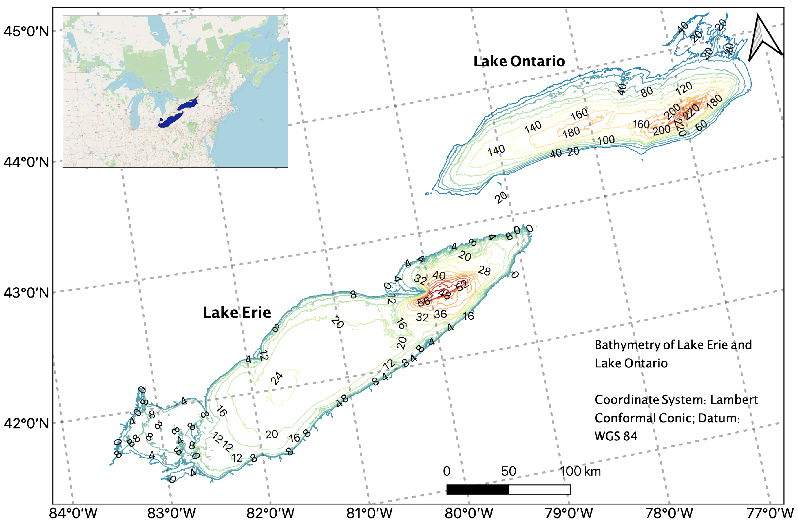
3.1. Study Area
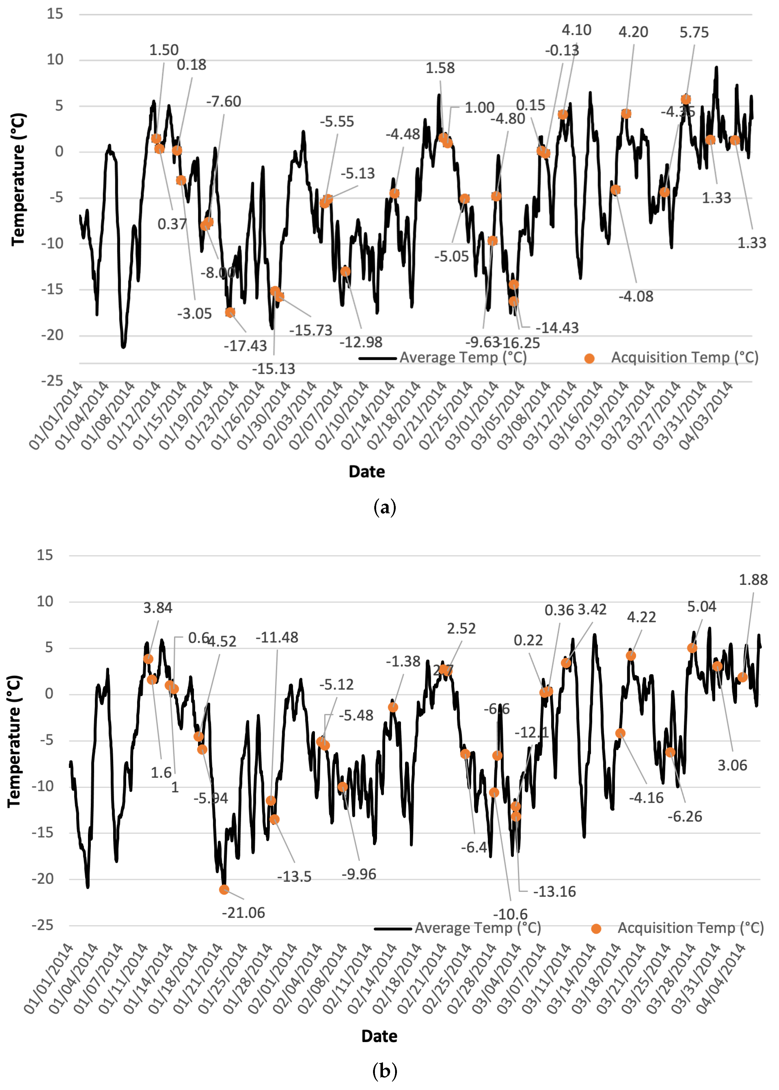
3.2. SAR Imagery
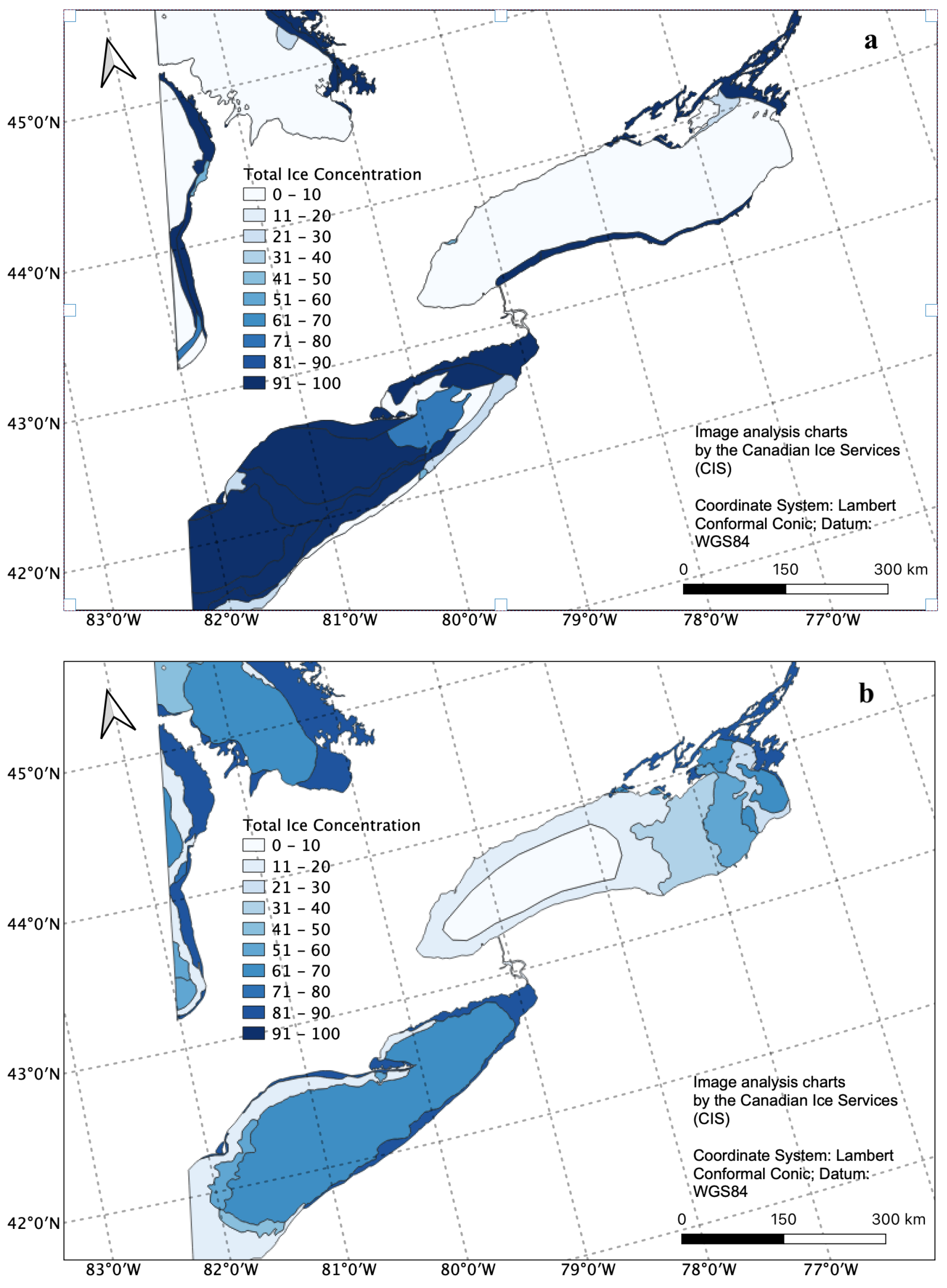
3.3. Image Analysis Charts
3.4. Data Processing
4. Methodology
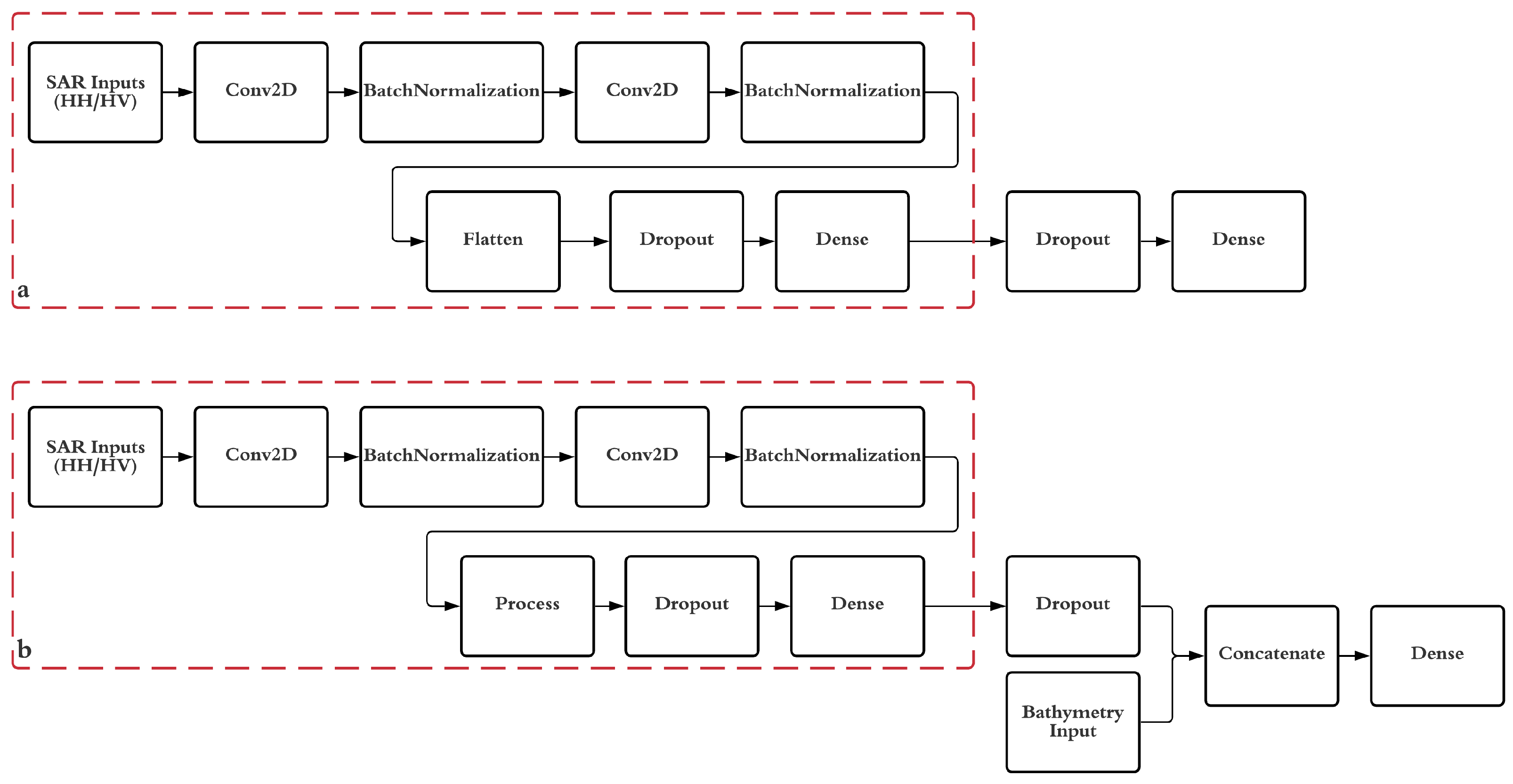
4.1. CNN Classification with a Custom Loss Function for Aleatoric Uncertainty Estimation
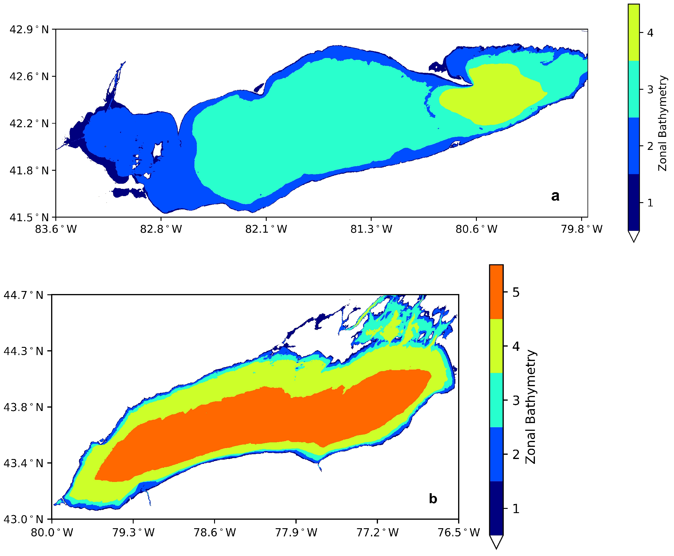
4.2. Incorporation of Bathymetry
4.3. CNN Architecture and Hyperparameter Selection
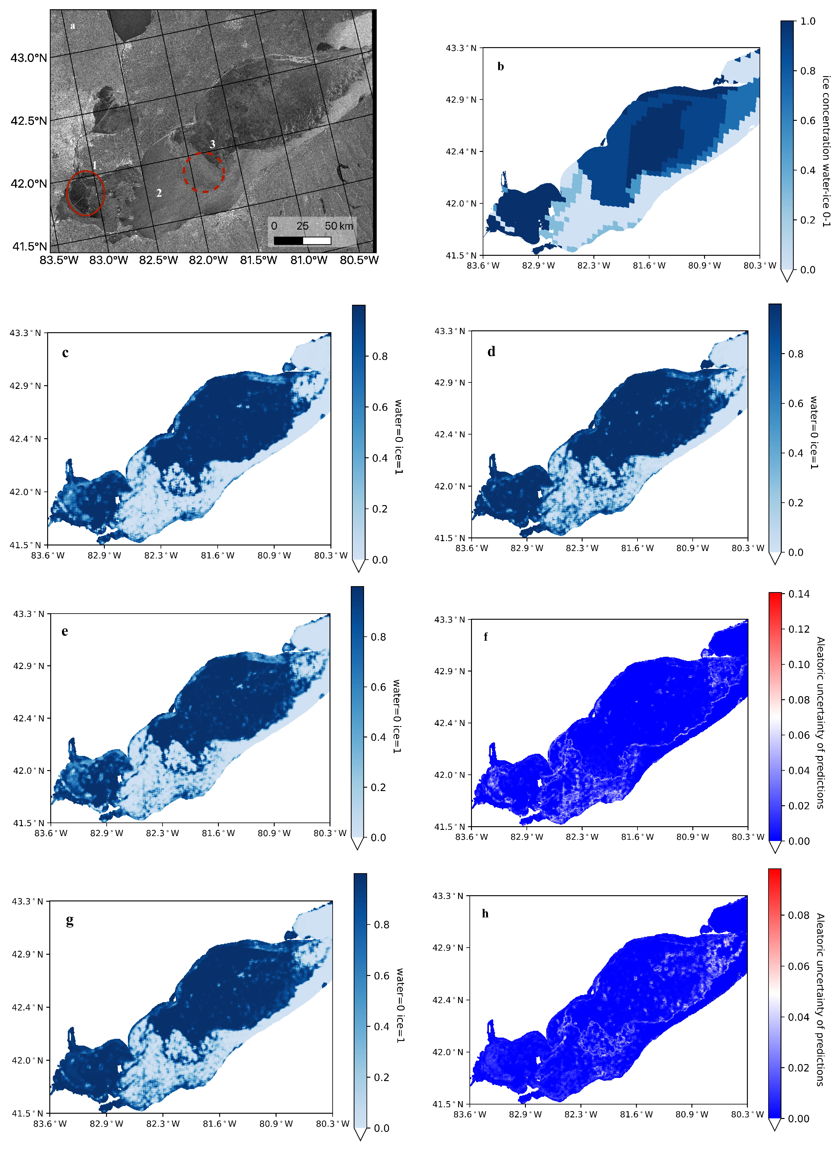
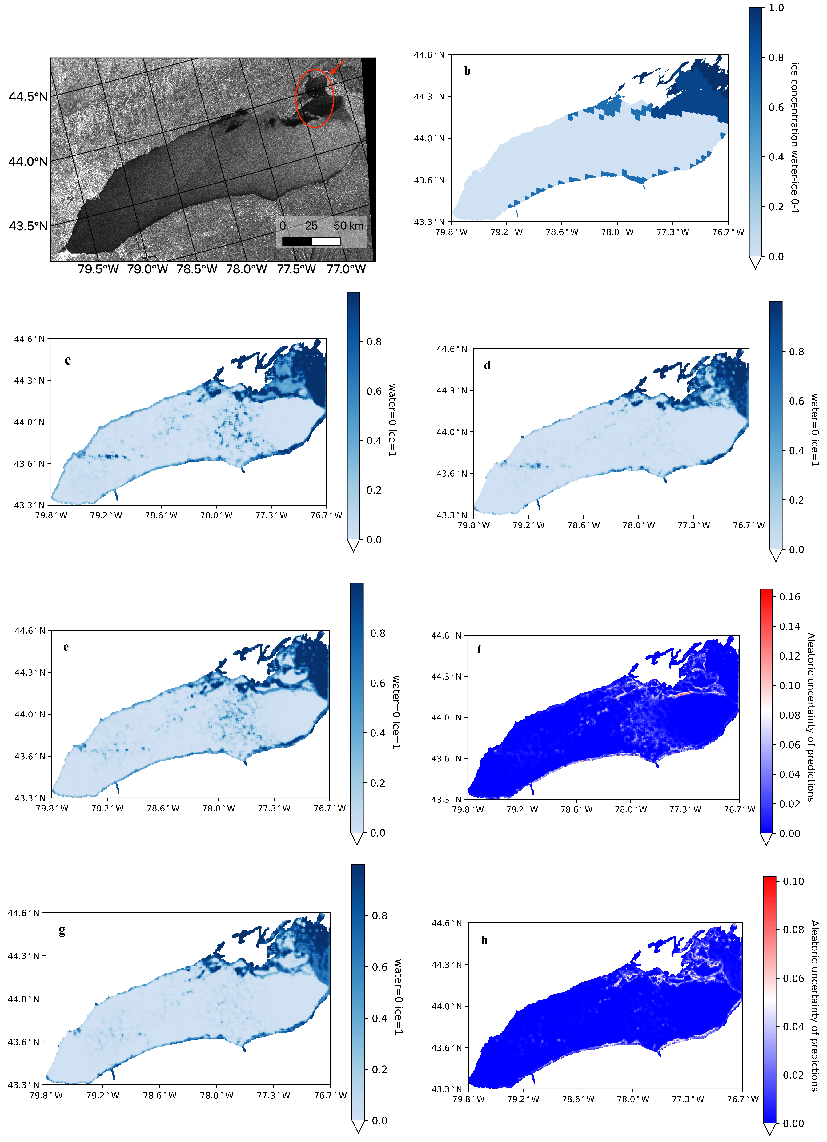
5. Results
6. Discussion
7. Conclusions
Author Contributions
Funding
Institutional Review Board Statement
Informed Consent Statement
Conflicts of Interest
References
- Pekel, J.F.; Cottam, A.; Gorelick, N.; Belward, A.S. High-resolution mapping of global surface water and its long-term changes. Nature 2016, 540, 418–422. [Google Scholar] [CrossRef] [PubMed]
- Duguay, C.R.; Prowse, T.D.; Bonsal, B.R.; Brown, R.D.; Lacroix, M.P.; Ménard, P. Recent trends in Canadian lake ice cover. Hydrol. Process. Int. J. 2006, 20, 781–801. [Google Scholar] [CrossRef]
- Brown, L.C.; Duguay, C.R. The response and role of ice cover in lake-climate interactions. Prog. Phys. Geogr. Earth Environ. 2010, 34, 671–704. [Google Scholar] [CrossRef]
- Baijnath-Rodino, J.A.; Duguay, C.R.; LeDrew, E. Climatological trends of snowfall over the Laurentian Great Lakes Basin. Int. J. Climatol. 2018, 38, 3942–3962. [Google Scholar] [CrossRef]
- Mironov, D.; Heise, E.; Kourzeneva, E.; Ritter, B.; Schneider, N.; Terzhevik, A. Implementation of the lake parameterisation scheme FLake into the numerical weather prediction model COSMO. Boreal Environ. Res. 2010, 15, 218–230. [Google Scholar]
- Minallah, S.; Steiner, A.L. The Effects of Lake Representation on the Regional Hydroclimate in the ECMWF Reanalyses. Mon. Weather Rev. 2021, 149, 1747–1766. [Google Scholar] [CrossRef]
- Nghiem, S.V.; Leshkevich, G.A. Satellite SAR remote sensing of Great Lakes ice cover, part 1. Ice backscatter signatures at C band. J. Great Lakes Res. 2007, 33, 722–735. [Google Scholar] [CrossRef]
- Gronewold, A.D.; Fortin, V.; Lofgren, B.; Clites, A.; Stow, C.A.; Quinn, F. Coasts, water levels, and climate change: A Great Lakes perspective. Clim. Chang. 2013, 120, 697–711. [Google Scholar] [CrossRef]
- Sterner, R.W.; Ostrom, P.; Ostrom, N.E.; Klump, J.V.; Steinman, A.D.; Dreelin, E.A.; Vander Zanden, M.J.; Fisk, A.T. Grand challenges for research in the Laurentian Great Lakes. Limnol. Oceanogr. 2017, 62, 2510–2523. [Google Scholar] [CrossRef]
- Manice, C. Manual of Standard Procedures for Observing and Reporting Ice Conditions. Environment Canada: Ottawa, ON, Canada, 2005. [Google Scholar]
- Deng, H.; Clausi, D. Unsupervised segmentation of synthetic aperture Radar sea ice imagery using a novel Markov random field model. IEEE Trans. Geosci. Remote Sens. 2005, 43, 528–538. [Google Scholar] [CrossRef]
- Sobiech, J.; Dierking, W. Observing lake- and river-ice decay with SAR: Advantages and limitations of the unsupervised k-means classification approach. Ann. Glaciol. 2013, 54, 65–72. [Google Scholar] [CrossRef] [Green Version]
- Wang, J.; Duguay, C.R.; Clausi, D.A.; Pinard, V.; Howell, S.E. Semi-automated classification of Lake Ice Cover using dual polarization RADARSAT-2 imagery. Remote Sens. 2018, 10, 1727. [Google Scholar] [CrossRef] [Green Version]
- Leigh, S.; Wang, Z.; Clausi, D.A. Automated Ice–Water Classification Using Dual Polarization SAR Satellite Imagery. IEEE Trans. Geosci. Remote Sens. 2014, 52, 5529–5539. [Google Scholar] [CrossRef]
- Hoekstra, M.; Jiang, M.; Clausi, D.A.; Duguay, C. Lake ice-water classification of RADARSAT-2 images by integrating IRGS Segmentation with pixel-based random forest labeling. Remote Sens. 2020, 12, 1425. [Google Scholar] [CrossRef]
- Ochilov, S.; Clausi, D.A. Operational SAR sea-ice image classification. IEEE Trans. Geosci. Remote Sens. 2012, 50, 4397–4408. [Google Scholar] [CrossRef]
- Geldsetzer, T.; van der Sanden, J.; Brisco, B. Monitoring lake ice during spring melt using RADARSAT-2 SAR. Can. J. Remote Sens. 2010, 36, S391–S400. [Google Scholar] [CrossRef]
- Karvonen, J. Baltic Sea Ice Concentration Estimation Based on C-Band Dual-Polarized SAR Data. IEEE Trans. Geosci. Remote Sens. 2014, 52, 5558–5566. [Google Scholar] [CrossRef]
- Dierking, W. Mapping of Different Sea Ice Regimes Using Images From Sentinel-1 and ALOS Synthetic Aperture Radar. IEEE Trans. Geosci. Remote Sens. 2010, 48, 1045–1058. [Google Scholar] [CrossRef]
- Zakhvatkina, N.; Korosov, A.; Muckenhuber, S.; Sandven, S.; Babiker, M. Operational algorithm for ice–water classification on dual-polarized RADARSAT-2 images. Cryosphere 2017, 11, 33–46. [Google Scholar] [CrossRef] [Green Version]
- Scott, K.A.; Xu, L.; Pour, H.K. Retrieval of ice/water observations from synthetic aperture radar imagery for use in lake ice data assimilation. J. Great Lakes Res. 2020, 46, 1521–1532. [Google Scholar] [CrossRef]
- Tom, M.; Aguilar, R.; Imhof, P.; Leinss, S.; Baltsavias, E.; Schindler, K. Lake ice detection from sentinel-1 sar with deep learning. ISPRS Ann. Photogramm. Remote Sens. Spat. Inf. Sci. 2020, 5, 409–416. [Google Scholar] [CrossRef]
- Wang, P.; Zhang, H.; Patel, V.M. SAR Image Despeckling Using a Convolutional Neural Network. IEEE Signal Process. Lett. 2017, 24, 1763–1767. [Google Scholar] [CrossRef] [Green Version]
- Lee, H.; Kwon, H. Going Deeper With Contextual CNN for Hyperspectral Image Classification. IEEE Trans. Image Process. 2017, 26, 4843–4855. [Google Scholar] [CrossRef] [Green Version]
- Jiang, T.; Cui, Z.; Zhou, Z.; Cao, Z. Data Augmentation with Gabor Filter in Deep Convolutional Neural Networks for Sar Target Recognition. In Proceedings of the IGARSS 2018—2018 IEEE International Geoscience and Remote Sensing Symposium, Valencia, Spain, 22–27 July 2018; pp. 689–692. [Google Scholar] [CrossRef]
- Kang, M.; Ji, K.; Leng, X.; Lin, Z. Contextual region-based convolutional neural network with multilayer fusion for SAR ship detection. Remote Sens. 2017, 9, 860. [Google Scholar] [CrossRef] [Green Version]
- Zhang, W.; Tang, P.; Zhao, L. Remote sensing image scene classification using CNN-CapsNet. Remote Sens. 2019, 11, 494. [Google Scholar] [CrossRef] [Green Version]
- Spreen, G.; Kaleschke, L.; Heygster, G. Sea ice remote sensing using AMSR-E 89-GHz channels. J. Geophys. Res. Ocean. 2008, 113, 1–14. [Google Scholar] [CrossRef] [Green Version]
- Boulze, H.; Korosov, A.; Brajard, J. Classification of sea ice types in sentinel-1 SAR data using convolutional neural networks. Remote Sens. 2020, 12, 2165. [Google Scholar] [CrossRef]
- Chen, F.C.; Jahanshahi, M.R. NB-CNN: Deep Learning-Based Crack Detection Using Convolutional Neural Network and Naïve Bayes Data Fusion. IEEE Trans. Ind. Electron. 2018, 65, 4392–4400. [Google Scholar] [CrossRef]
- Asadi, N.; Scott, K.A.; Komarov, A.S.; Buehner, M.; Clausi, D.A. Evaluation of a Neural Network With Uncertainty for Detection of Ice and Water in SAR Imagery. IEEE Trans. Geosci. Remote Sens. 2021, 59, 247–259. [Google Scholar] [CrossRef]
- Kendall, A. Geometry and Uncertainty in Deep Learning for Computer Vision. Ph.D. Thesis, University of Cambridge, Cambridge, UK, 2019. [Google Scholar]
- Hüllermeier, E.; Waegeman, W. Aleatoric and epistemic uncertainty in machine learning: An introduction to concepts and methods. Mach. Learn. 2021, 110, 457–506. [Google Scholar] [CrossRef]
- Great Lakes Environmental Research Laboratory—Historical Ice Cover. Available online: https://www.glerl.noaa.gov/data/ice/#historical (accessed on 30 September 2020).
- Historical Climate Data. Available online: https://climate.weather.gc.ca/historical_data/search_historic_data_e.html (accessed on 30 September 2020).
- Kendall, A.; Gal, Y. What uncertainties do we need in Bayesian deep learning for computer vision? arXiv 2017, arXiv:1703.04977. [Google Scholar]
- Edinger, J.E.; Duttweiler, D.W.; Geyer, J.C. The response of water temperatures to meteorological conditions. Water Resour. Res. 1968, 4, 1137–1143. [Google Scholar] [CrossRef]
- Williams, S.G.; Stefan, H.G. Modeling of lake ice characteristics in North America using climate, geography, and lake bathymetry. J. Cold Reg. Eng. 2006, 20, 140–167. [Google Scholar] [CrossRef]
- Riseng, C.M.; Wehrly, K.E.; Wang, L.; Rutherford, E.S.; McKenna, J.E.; Johnson, L.B.; Mason, L.A.; Castiglione, C.; Hollenhorst, T.P.; Sparks-Jackson, B.L.; et al. Ecosystem classification and mapping of the laurentian great lakes. Can. J. Fish. Aquat. Sci. 2018, 75, 1693–1712. [Google Scholar] [CrossRef] [Green Version]
- Loshchilov, I.; Hutter, F. SGDR: Stochastic gradient descent with warm restarts. In Proceedings of the 5th International Conference on Learning Representations, ICLR 2017—Conference Track Proceedings, Toulon, France, 24–26 April 2017; pp. 1–16. [Google Scholar]


| Acquisition Date | Acquisition Time | Lake Erie | Lake Ontario | ||||
|---|---|---|---|---|---|---|---|
| Train | Test | Evaluation | Train | Test | Evaluation | ||
| 11 January 2014 | 23:15 | ||||||
| 12 January 2014 | 11:26 | ||||||
| 14 January 2014 | 23:27 | ||||||
| 15 January 2014 | 11:40 | ||||||
| 18 January 2014 | 23:11 | ||||||
| 19 January 2014 | 11:22 | ||||||
| 22 January 2014 | 11:35 | ||||||
| 28 January 2014 | 23:19 | ||||||
| 29 January 2014 | 11:31 | ||||||
| 4 February 2014 | 23:15 | ||||||
| 5 February 2014 | 11:26 | ||||||
| 7 February 2014 | 23:27 | ||||||
| 14 February 2014 | 23:23 | ||||||
| 21 February 2014 | 23:19 | ||||||
| 22 February 2014 | 11:31 | ||||||
| 25 February 2014 | 11:44 | ||||||
| 28 February 2014 | 23:15 | ||||||
| 1 March 2014 | 11:26 | ||||||
| 3 March 2014 | 23:27 | ||||||
| 4 March 2014 | 11:40 | ||||||
| 7 March 2014 | 23:11 | ||||||
| 8 March 2014 | 11:22 | ||||||
| 10 March 2014 | 23:23 | ||||||
| 18 March 2014 | 11:31 | ||||||
| 20 March 2014 | 23:31 | ||||||
| 25 March 2014 | 11:26 | ||||||
| 28 March 2014 | 11:40 | ||||||
| 1 April 2014 | 11:22 | ||||||
| 4 April 2014 | 11:34 | ||||||
| Model Predictions | Ice Chart | ||
|---|---|---|---|
| Ice | Water | Marginal Total | |
| Ice | a | b | a + b |
| Water | c | d | c + d |
| Marginal Total | a + c | b + d | a + b + c + d = n |
| proportion correct ice = a/(a + c) proportion correct water = d/(b + d) total proportion correct = (a + d)/n missed ice = c/(c + d) false alarm (missed water) = b/(a + b) | |||
| Model | Proportion Scores | ||||
|---|---|---|---|---|---|
| Correct Ice | Correct Water | Total Correct | Missed Ice | Missed Water | |
| Baseline CNN (inputs: HH-HV) | 0.991 | 0.468 | 0.967 | 0.293 | 0.025 |
| CNN with bathymetry (inputs: HH, HV, bathymetry) | 0.992 | 0.400 | 0.969 | 0.179 | 0.025 |
| CNN with aleatoric loss (inputs: HH, HV) | 0.992 | 0.467 | 0.968 | 0.261 | 0.025 |
| CNN with aleatoric loss and bathymetry (inputs: HH, HV, bathymetry) | 0.996 | 0.421 | 0.970 | 0.160 | 0.027 |
| Model | Proportion Scores | ||||
|---|---|---|---|---|---|
| Correct Ice | Correct Water | Total Correct | Missed Ice | Missed Water | |
| Baseline CNN (inputs: HH, HV) | 0.965 | 0.763 | 0.819 | 0.017 | 0.390 |
| CNN with bathymetry (inputs: HH, HV, bathymetry) | 0.910 | 0.870 | 0.881 | 0.038 | 0.272 |
| CNN with aleatoric loss (inputs: HH, HV) | 0.949 | 0.760 | 0.812 | 0.025 | 0.397 |
| CNN with aleatoric loss and bathymetry (inputs: HH, HV, bathymetry) | 0.918 | 0.840 | 0.862 | 0.036 | 0.313 |
Publisher’s Note: MDPI stays neutral with regard to jurisdictional claims in published maps and institutional affiliations. |
© 2022 by the authors. Licensee MDPI, Basel, Switzerland. This article is an open access article distributed under the terms and conditions of the Creative Commons Attribution (CC BY) license (https://creativecommons.org/licenses/by/4.0/).
Share and Cite
Saberi, N.; Scott, K.A.; Duguay, C. Incorporating Aleatoric Uncertainties in Lake Ice Mapping Using RADARSAT–2 SAR Images and CNNs. Remote Sens. 2022, 14, 644. https://doi.org/10.3390/rs14030644
Saberi N, Scott KA, Duguay C. Incorporating Aleatoric Uncertainties in Lake Ice Mapping Using RADARSAT–2 SAR Images and CNNs. Remote Sensing. 2022; 14(3):644. https://doi.org/10.3390/rs14030644
Chicago/Turabian StyleSaberi, Nastaran, Katharine Andrea Scott, and Claude Duguay. 2022. "Incorporating Aleatoric Uncertainties in Lake Ice Mapping Using RADARSAT–2 SAR Images and CNNs" Remote Sensing 14, no. 3: 644. https://doi.org/10.3390/rs14030644
APA StyleSaberi, N., Scott, K. A., & Duguay, C. (2022). Incorporating Aleatoric Uncertainties in Lake Ice Mapping Using RADARSAT–2 SAR Images and CNNs. Remote Sensing, 14(3), 644. https://doi.org/10.3390/rs14030644