Passive Microwave Melt Onset Retrieval Based on a Variable Threshold: Assessment in the Canadian Arctic Archipelago


1
Department of Systems Design Engineering, University of Waterloo, Waterloo, ON N2L 3G1, Canada
2
Department of Geography, University of Victoria, Victoria, BC V8P 5C2, Canada
*
Author to whom correspondence should be addressed.
†
These authors contributed equally to this work.
Remote Sens. 2019, 11(11), 1304; https://doi.org/10.3390/rs11111304
Submission received: 25 April 2019
/
Revised: 22 May 2019
/
Accepted: 28 May 2019
/
Published: 31 May 2019
Abstract
:The Canadian Arctic Archipelago (CAA) presents unique challenges to the determination of melt onset (MO) using remote sensing data. High spatial resolution data is required to discern melt onset among the islands and narrow waterways of the region. Current passive microwave retrievals use daily averaged 19 GHz and 37 GHz data from the multi-channel microwave radiometer (SMMR) and/or the special sensor microwave/imager (SSM/I). The development of a new passive microwave melt onset method capable of using higher resolution data is desirable. The new passive microwave melt onset method described here, named the Dynamic Threshold Variability Method (DTVM), uses higher resolution data from the 37 GHz vertically-polarized channel from the advanced microwave scanning radiometers (AMSR-E and AMSR-2). The DTVM MO detection methodology differs from previously presented passive microwave Arctic MO methods in that it does not use a fixed threshold of a brightness temperature parameter. Instead, the DTVM determines MO dates based on the distribution of dates corresponding to the exceedance of a range of brightness temperature variability thresholds. The method also uses swath data instead of daily averaged brightness temperatures, which is found to lead to improved melt detection. Two current passive microwave MO methods are compared and evaluated for applicability in the CAA alongside the DTVM. The DTVM provides MO dates at a higher spatial resolution than earlier methods in addition to higher correlation with MO dates from surface air temperature (SAT) reanalyses. It is found that, for some years, MO dates in the CAA exhibit a latitudinal dependence, while in other years the MO dates in the CAA are relatively uniform across the domain.
1. Introduction
Melt onset (MO) indicates a transition from winter to spring and is an important component of the Arctic sea ice energy balance [1,2]. During melt, the sea-ice or snow surface becomes wet, causing a reduction of surface albedo. The MO date is therefore representative of an initiation of a positive feedback loop. The reduced albedo allows for greater absorption of shortwave solar radiation, which can lead to increased surface melt [3]. During melt, as the ice begins to break-up, the appearance of open water leads to increased absorption of solar radiation into the ocean, which can both accelerate bottom melt and delay freeze-up [4,5]. Melt onset dates are therefore correlated with melt season length [6], and the September minimum sea ice extent, making long term MO information of value for climate studies [7].
The Canadian Arctic Archipelago (CAA) is a region of islands in the Canadian Arctic between the Arctic Ocean and the Hudson Bay System. The ice cover in the CAA is a mixture of first-year ice, and thicker multi-year ice. In the CAA, the duration of the melt season is linked with the quantity of first-year ice that remains at the end of the ice season, and is therefore promoted to multi-year ice [8]. Due to the thickness of multi-year ice, it is less likely to break-up during melt than first-year ice. However, during melt the thickness of the multi-year ice may be decreased, impacting its ability to survive future melt seasons [8]. Melt onset and the duration of the melt season in the CAA are therefore particularly important toward understanding the fraction and characteristics of multi-year ice in the CAA. Due to the narrow waterways of the CAA, high-resolution satellite data are often used to determine MO in this region.
Data from synthetic aperture radars (SARs), scatterometers and passive microwave radiometers have been used in previous studies to determine MO dates [8,9,10,11,12]. While data from both SARs and scatterometers can yield MO dates at reasonably high spatial resolution (100 m–5 km), the most commonly used MO retrieval methods use passive microwave data from the scanning multi-channel microwave radiometer (SMMR), and/or the special sensor microwave/imager (SSM/I), or the special sensor microwave imager/sounder (SSMIS). These passive microwave data are available each day over the entire Arctic from 1979 to the present, making these data ideal for climate studies. Current passive microwave MO estimation methods include the advanced horizontal range algorithm (AHRA), developed by Drobot and Anderson in 2001 [13], and the passive microwave algorithm (PMW) developed by Markus in 2009 [7]. Both methods use daily averaged 19 GHz and 37 GHz brightness temperature data from SMMR and SSM/I. However, the instrument field of view (IFOV) of the SSM/I sensor is 69 × 43 km for the 19 GHz channel, with similar IFOV for SMMR. These IFOVs are too large to resolve MO dates for large portions of the CAA without significant signal contamination due to land. Since 2002, advanced microwave scanning radiometers (AMSR-E and AMSR-2) have been collecting data over the arctic region at a much higher spatial resolution. For example, for the 19 GHz channel on AMSR2 the IFOV is 14 × 22 km, while for the 36.5 GHz channel (hereafter 37 GHz) it is 12 × 7 km. The IFOVs are similar for the AMSR-E instrument. Given these significantly smaller IFOVs, it is logical for MO in the CAA to be determined using the higher resolution AMSR data rather than the lower resolution SMMR and SSM/I data, at the expense of a shorter time series. In addition, it would be advantageous to utilize only the 37 GHz channel if possible. In this regard, the method developed in [14] for MO over the Greenland ice sheet is of interest. This method uses the brightness temperature difference between ascending and descending passes at 37 GHz. When this difference exceeds a certain threshold, MO is said to have occurred. A drawback of this approach (and others) is that the threshold used to determine MO is fixed, and needs to be re-calibrated for specific geographic regions [14]. Ideally, a method that does not rely on a fixed threshold could be used.
In this paper, we present a new MO determination method, named the dynamic threshold variability method (DTVM). Similar to [14], the method uses swath data to pick up on diurnal variability patterns associated with MO [15] that would otherwise be missed using daily averaged data, which are used in the AHRA and PWM algorithms. In this sense, our method is designed to detect early melt onset, which corresponds to the first appearance of water in the snowpack and is often followed by diurnal cycles of melt and refreeze [7,16]. An early melt onset date is similarly defined in the PMW algorithm, while AHRA has a single MO date. Details pertaining to the MO detection of these two methods can be found in [7,13]. The main difference between DTVM and previous approaches is that instead of using a fixed threshold, a range of threshold values are evaluated. To present this new approach, we first review the two leading MO methods for passive microwave data; the AHRA and PMW methods. We then describe the methodology used in the DTVM for MO estimation. This is followed by a comparison of the passive microwave methods with each other, in addition to MO estimated using 2 m air temperature from reanalysis as well as data from temperature profilers installed in sea ice. Finally, we discuss benefits and possible shortcomings of the DTVM that can be improved upon in future studies.
2. Study Region and Data
2.1. Study Region
The CAA is a region of islands located north of mainland Canada. The National Snow and Ice Data Center (NSIDC) definition of the CAA used in previous studies has been chosen as the study region. An outline of the region of interest is provided in Figure 1. The application of passive-microwave based sea ice monitoring methods and climate models to the CAA is challenging due to difficulties resolving narrow passages and bays. The CAA contains a mixture of first-year (FYI) and multi-year (MYI) ice, with multi-year ice generally being thicker and more resistant to melt than first-year ice. Trends in ice cover and melt season duration in the CAA often do not follow those in the central Arctic. This is due in part to the the flux of MYI in and out of the domain [8] as well as the potential role of the land surface warming. Melt onset in the CAA is of particular interest for shipping as the region contains the Northwest Passage. The use of MO as an indicator of ice break-up may also be of interest to local communities.
2.2. Brightness Temperature Data
For the estimation of MO, brightness temperature data from AMSR-E and AMSR2 were used. For each date in the study period, all available brightness temperature swaths in the study region were obtained and interpolated to a Northern Hemisphere polar stereographic grid using nearest neighbour interpolation. The AMSR-E data were acquired from the NSIDC while AMSR2 data were accessed directly from the Japan Aerospace Exploration Agency (JAXA). All brightness temperature data used were L2 swath re-sampled brightness temperature products. No additional calibration was necessary to bring the AMSR2 brightness temperatures into agreement with those from AMSR-E because the DTVM method (described in Section 3) uses a dynamic threshold and therefore does not rely on a specified value of brightness temperature parameter. For determination of MO, the swath data were regridded to a common grid. Three Northern Hemisphere polar stereographic grids are available from NSIDC at 25 km, 12.5 km and 6 km nominal grid spacing (NSIDC). For comparison with MO from AHRA and PMW [7,12], MO dates were determined using the 25 km NSIDC grid. An additional set of MO dates were estimated using AMSR2 data on the 6 km grid. Note that there is a gap in data between when the AMSR-E sensor failed (25 October 2011) and when data are available from AMSR2 (4 July 2012). Hence, no MO dates are calculated for 2012.
AMSR data is released with a land-flag to indicate the degree to which the brightness temperature at a pixel is influenced by land. To avoid land contamination, the nearest neighbour interpolation used to map the AMSR data to the NSIDC grids does not consider points with any land contamination. Therefore, grid points near land may not have the closest brightness temperature data but rather will have the brightness temperature data of the nearest point within 10 km with no land contamination. We note that this is approximate, since there are many small islands that are not represented in the landmask, and the instrument field of view is not exact due to the motion of the antenna and the spacecraft [17].
2.3. Arctic System Reanalysis Data
Surface air temperature (SAT) MO dates were calculated using 2 m air temperature from the surface analyses of the Arctic system reanalysis (ASR) [18]. These data are provided by the National Center for Atmospheric Research (NCAR). The ASR data were chosen because the spatial resolution (15 km) is similar to that of the passive microwave data, and the 2 m air temperature is less biased than that from ERA Interim in a comparison with air temperature from weather stations [18]. We note that ASR utilizes observational data in addition to prognostic model calculations to obtain the state of the atmosphere. In particular, ASR assimilates ice concentration derived from passive microwave data. Since our study region is mostly ice-covered for the season of interest (100% ice concentration), this likely does not have a significant impact on our results. To verify this, an additional set of MO estimates were made, excluding points where ice concentration from the ARTIST sea ice (ASI) algorithm [19] was less than 90%. It was found that this had a negligible impact on the MO dates.
2.4. Temperature Profiler Data
Air temperature and snow/ice interface temperature data from Ocean Networks Canada (ONC) were used in the comparison of passive microwave MO methods. The data from ONC were collected from 908 IceTemp profilers produced by Oceanetic Measurement. The temperature profilers recorded air temperature, surface temperature (at the snow/ice interface) as well as a series of temperatures at 50 cm depth intervals through the ice profile. The profilers were deployed during wintertime conditions and remained in the ice cover through the period of interest, generally until the end of June. The profilers sent data at hourly intervals with a rated accuracy of 0.1 C. The profilers were supported by three arms that ensured that the thermistors remained at a correct level with respect to the snow/ice interface [20]. The snow/ice interface temperature (here-after surface temperature) was recorded by a thermistor located just below the snow/ice interface. The air temperature was recorded by the thermistor located above the profiler, approximately 50 cm above the ice surface (at deployment), and above the snowpack. Location data was also recorded by the profilers, but for the period of interest the movement of the profilers was minimal. All of the profiler data used were from installations on first year ice.
2.5. MO Data
AHRA MO data is available from NSIDC for the years 1979–2012. These MO dates are computed using brightness temperatures from SMMR and SSM/I-SSMIS. PMW MO dates are available from 1979–2018, and also are computed using brightness temperatures from SMMR and SSM/I-SSMIS. Both PMW and AHRA data sets are available at the 25 km NSIDC grid resolution [7].
3. MO Detection Methods
Brightness temperature data from passive microwave data are particularly well suited for analysis of surface conditions during melt as these data are generally insensitive to atmospheric conditions (for lower frequencies) and the signals are very responsive to surface changes caused by melt. Previous MO algorithms have included AHRA developed by Drobot and Anderson [13] and the PMW algorithm, developed by Markus [7].
3.1. Advanced Horizontal Range Algorithm (AHRA)
The AHRA uses the difference between the horizontally polarized brightness temperature at 19 GHz (TB19H) and the horizontally polarized brightness temperature at 37 GHz (TB37H) to detect MO. The algorithm works on the premise that during the winter, TB37H is lower than TB19H due to increased scattering from the snow cover. During early melt, the presence of water in the snowpack leads to an emissivity increase that is greater for TB37H than TB19H Ghz [13]. The horizontal range parameter, HR, is defined as TB19H subtracted by TB37H. The AHRA uses both a discrete threshold on HR and a 20 day window test range to determine MO as follows: MO is assigned on the first day of the year on which the HR parameter drops below K; for days with an HR value between 4 K and −10 K, the algorithm will also define MO on a day when the range of HR values for 10 days after and including test day is more than 7.5 K greater than the range of values for the 10 days before the test day. The latter part of the algorithm is called the 20-day window test. As a result of the 20-day window test, the AHRA can determine melt up to 9 days before melt characteristics are detectable with the HR parameter [21]. The AHRA has been applied to daily averaged brightness temperature data from SMMR and SSM/I to derive a long term record of MO dates for the arctic from 1979–2012 [22]. Due to the fixed thresholds used by the AHRA, the method is dependent on the calibration of the sensor. Brightness temperature data from different sensors that have not been inter-calibrated may produce inconsistent MO dates using the AHRA.
3.2. Passive Microwave Algorithm (PMW)
The PMW algorithm determines dates for early melt onset (EMO), continuous melt onset (CMO) as well as freeze up and early freeze up. Similarly to the AHRA, the PMW uses brightness temperature data from both the 19 GHz and 37 GHz channels. Unlike AHRA, which uses only a single parameter (HR), the PMW algorithm uses multiple parameters, each sensitive to a different component of melt and freeze onset [7]. Parameters include the absolute value of the daily change in 37 GHz vertically polarized brightness temperature, the day to day variability of the vertical gradient ratio of the two channels as well as a linear combination of the vertical polarization of the two channels [23]. These parameters are combined in a weighted sum to create a daily time series for the year. CMO is determined to be the date with the maximum value of this sum over the melt season, while EMO is determined to be the day with the second maximum within the melt season. A neighbourhood check is performed on pixels as part of the PMW method to ensure spatial continuity of the MO dates. In some cases, the PMW may not define an EMO date [7]. This may be caused by EMO and MO occurring on the same day. EMO dates defined using the PMW method are more consistent with MO dates defined by the AHRA than the CMO dates [21]. The PMW algorithm has been applied to daily averaged brightness temperature data from SMMR and SSM/I to derive a long term record of MO dates for the arctic from 1979–2018 [7]. For the comparisons carried out in this paper, only the EMO values from the PMW algorithm will be used.
3.3. DTVM
The DTVM method has been primarily developed to detect MO at a higher spatial resolution than previous passive microwave methods. The DTVM achieves this by using only vertically polarized 37 GHz (TB37V) data from the AMSR-E and AMSR2 instruments. DTVM also differs from previous passive microwave MO methods in its use of swath data, and in that it avoids using fixed thresholds. The motivation to use the 37 GHz channel is based on the spatial resolution this channel provides, its sensitivity to the presence of liquid water in the snow cover, and its relative insensitivity to atmospheric moisture. For dry snow, microwave emission at higher frequencies (shorter wavelengths) is reduced due to volume scattering from snow grains [24]. This reduction is more noticeable for 37 GHz as compared to 19 GHz, and contrasts with the high emission when liquid water is present. It is this contrast that indicates MO [7,13]. While 89 GHz can provide even higher spatial resolution than 37 GHz, this frequency is too sensitive to atmospheric moisture to allow it to be used for MO detection (this was also noted in [24]).
DTVM expands on the premise used by the PMW algorithm, where an increase in the absolute value of the day-to-day change in TB37V is indicative of melt. Instead of using the day to day difference in TB37V, as with the PMW algorithm, the DTVM creates a time series of TB37V variability, where the variability is computed as the standard deviation of TB37V over a specified number of days. For results shown here, for each day of the year, the standard deviation is determined using the TB37V values from the day in question as well as the two previous days. The resulting time series of variability is then used to determine an appropriate MO date. At most locations in the study region there are between 2 and 4 usable swaths for each day of the year. Therefore, the variability series is calculated using the standard deviation of between 6 and 12 TB37V values. Higher latitudes may have more than 4 usable swaths in a given day.
Many MO estimation methods [9,21] use fixed thresholds of the MO parameter. These methods generally operate by choosing the first day at which the threshold is exceeded as the MO date. To enable a more robust detection of MO, an approach using a dynamic threshold has been developed in the present study. The approach uses a range of thresholds to determine a distribution of potential MO dates. This distribution is then used to determine the most likely MO date and a corresponding measure of confidence.
The dynamic threshold approach for MO determination can be broken down into 5 steps as follows:
- The time series of variability is created from at least the first day of the year until the end of the possible melt season. The variability is calculated using brightness temperatures over a given range, which includes the day of interest and the two prior days.
- A range of thresholds is created, varying from 0 to the maximum value of variability within the time series.
- MO dates are determined for each possible threshold between 0 and the maximum value of the time series. MO dates outside of the possible melt range (day of year 61 to 200) are discarded. If there are more MO dates before the melt range than there are within it, then no MO date will be defined.
- The inter-quartile range (IQR) is determined from the range of remaining MO dates. The IQR is calculated by taking the 75th percentile value from the MO dates and subtracting it from the 25th percentile value. A small IQR value indicates a very well defined MO date, whereas a very large IQR value indicates a poorly defined MO date. If the IQR for the given pixel is larger than a specified value (20 was used here), a MO onset date is not estimated for that pixel.
- Finally, the MO date is defined as the date corresponding to the 25th percentile.
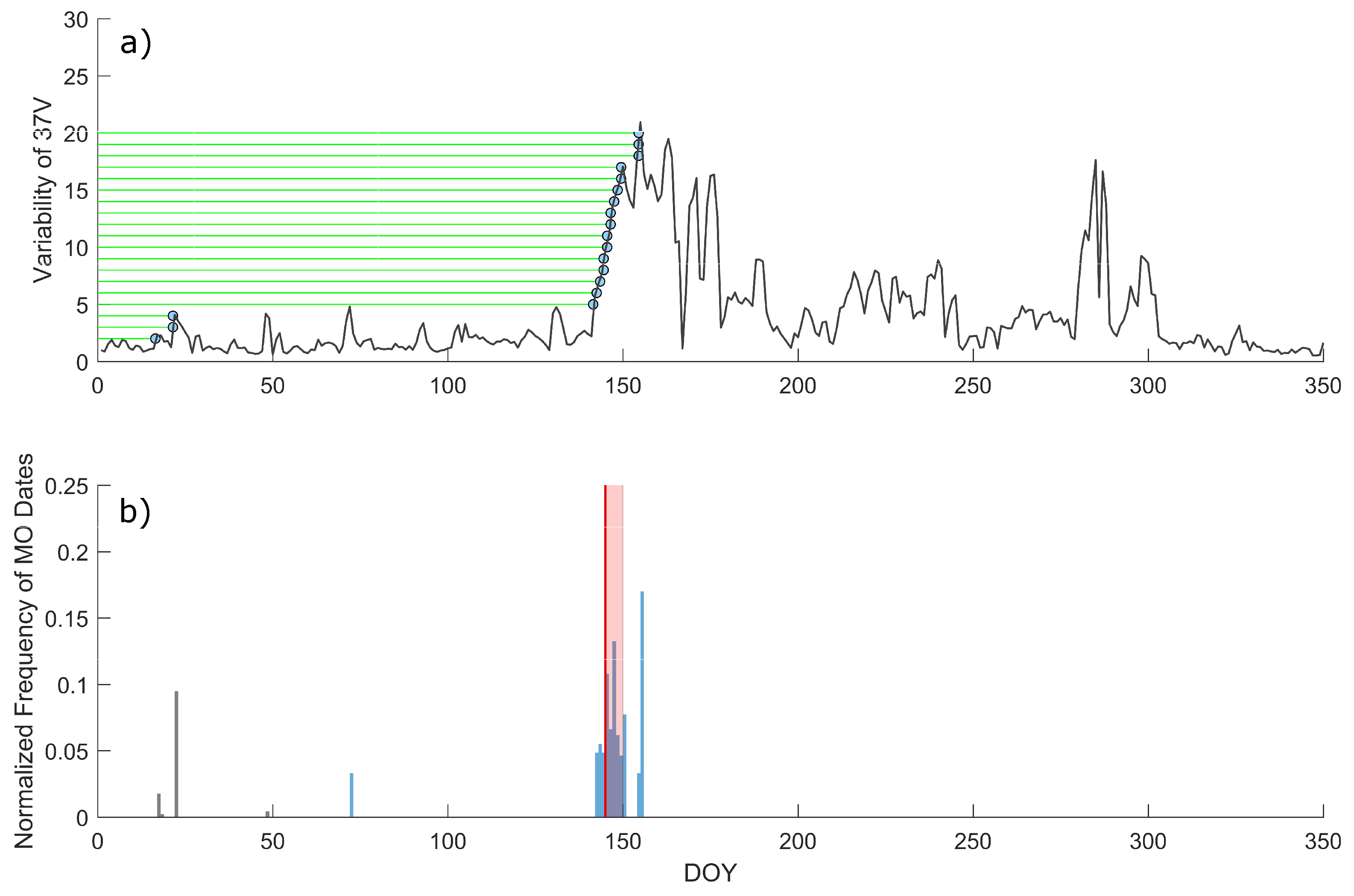
An example of the estimation of MO using DTVM is provided in Figure 2. Note that the DTVM applies the dynamic threshold approach to the variability of TB37V. The dynamic threshold approach can also be applied to other parameters, such as the HR parameter or brightness temperatures from other channels. When applying the dynamic threshold approach, the number of thresholds used, the dates used to define the melt period and the acceptable IQR value can be varied. Melt onset dates used in this report were obtained using 500 different threshold values, a melt range defined from DOY 61 to DOY 200 and an IQR maximum of 20 days. The start of the melt range was defined as DOY 61 to match the start date of AHRA method [21]. The end of the melt range was defined as DOY 200 as this is a reasonable maximum MO date for the CAA. The IQR maximum of 20 days was chosen based on comparisons with other potential IQR maximums. Large IQR maximums do not filter out poorly defined MO dates and small IQR maximums may filter more gradual, but still well defined MO signals. The number of different threshold values to test was chosen to enable the MO date quartiles to be well defined. For the results presented here, 500 threshold values were considered.
Due to the use of swath data, the DTVM may be picking up on diurnal variability associated with melt that is otherwise missed by methods using daily averaged data. This potentially makes the DTVM more effective at determining MO. Figure 3 shows the application of the DTVM to swath data as compared to daily averaged data. Significant TB fluctuations, likely due to MO, can be seen in both sets of TB data, although they are more pronounced in the swath data. The MO date estimated from the swath data is closer to the onset of these fluctuations, whereas the MO date estimated from the daily averaged data is several days later.
3.4. Estimation of MO Using SAT
The appearance of water in the snowpack, indicating the onset of melt, is often correlated with an increase in SAT, where the SAT is taken to be the 2 m air temperature either from an in-situ observation [1,2,25] or from a surface analysis based on a weather forecasting model [26]. In an earlier study [12], AHRA MO dates were compared to those estimated by thresholding SAT using various methods, which we have also adopted here. These methods are as follows:
- 14 day averaged SAT values were used with −1 °C threshold.
- Daily averaged SAT values were used with −1 °C threshold.
- Daily averaged SAT values were used with 0 °C threshold.
For this comparison both daily and 14 day averaged SAT data were used over a range of SAT thresholds. In [12], SATs were obtained from both buoy data and data from the atmospheric infrared sounder (AIRS). The latter SAT is an interpolated air temperature using the AIRS temperature profiles and surface pressure. In our study AIRS data were not utilized because the spatial resolution of the SAT product is 1° × 1°, which is too coarse for analysis in the CAA.
4. Results
4.1. Comparison of Passive Microwave MO Methods
The three passive microwave methods described in Section 3, AHRA, PMW and DTVM, are compared and evaluated for their applicability to MO estimation in the CAA. Note that the overlap between AMSR-E data and available data for PMW and AHRA MO dates, is from 2003 to 2011. There was a total of 6147 points over the 9 years of data that were used to compare MO between the methods. The number of points available on any given year varies because at each grid point, a MO date must be available from all three methods for that grid point to be used in statistical comparisons.
A spatial comparison of MO dates from the three passive microwave MO estimation methods for a representative year is provided in Figure 4. It can be seen that the three methods are in agreement over a large part of the CAA, with some differences in the Amundsen Gulf and Coronation Gulf. In panel (d) the MO dates are shown for DTVM at 6 km for comparison with those from 25 km, shown in panel (c). As expected, finer regional details can be seen at the higher spatial resolution.
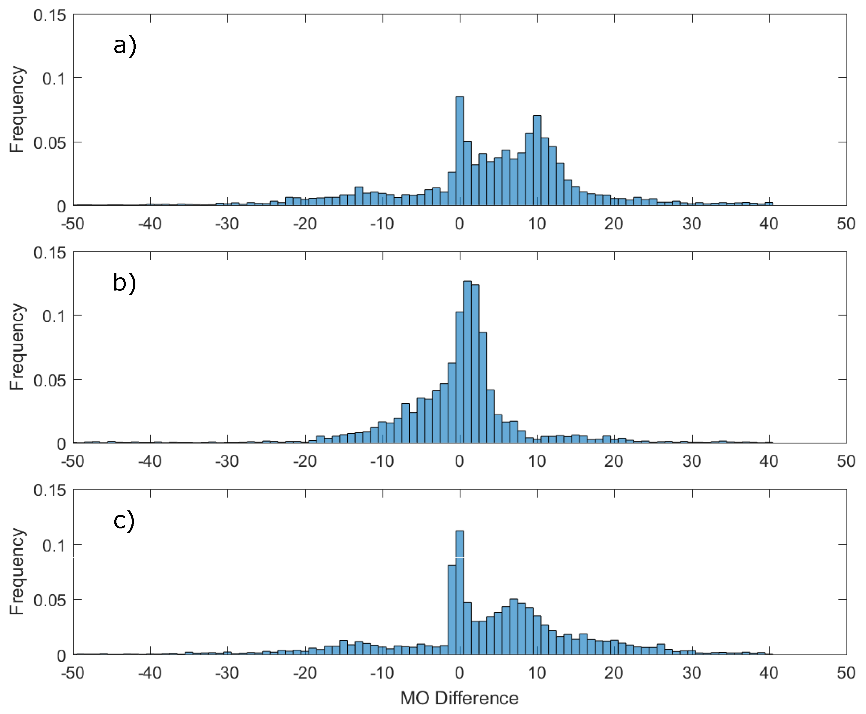
Histograms displaying pixel-wise differences in the MO dates are provided in Figure 5. The DTVM and the PMW method show a general agreement for most points with the DTVM flagging some points earlier than the PMW EMO (large negative tail in Figure 5b). Comparisons between AHRA MO dates and both PMW and DTVM MO dates show bi-modal distributions. The modes of these distributions are centered around −1:1 and 8:10. The first mode indicates a general agreement between the methods, while the second mode is likely caused by the AHRA algorithm flagging melt early due to the 20-day window test. The differences between the three methods are summarized in Table 1.
4.2. SAT MO Dates Comparison
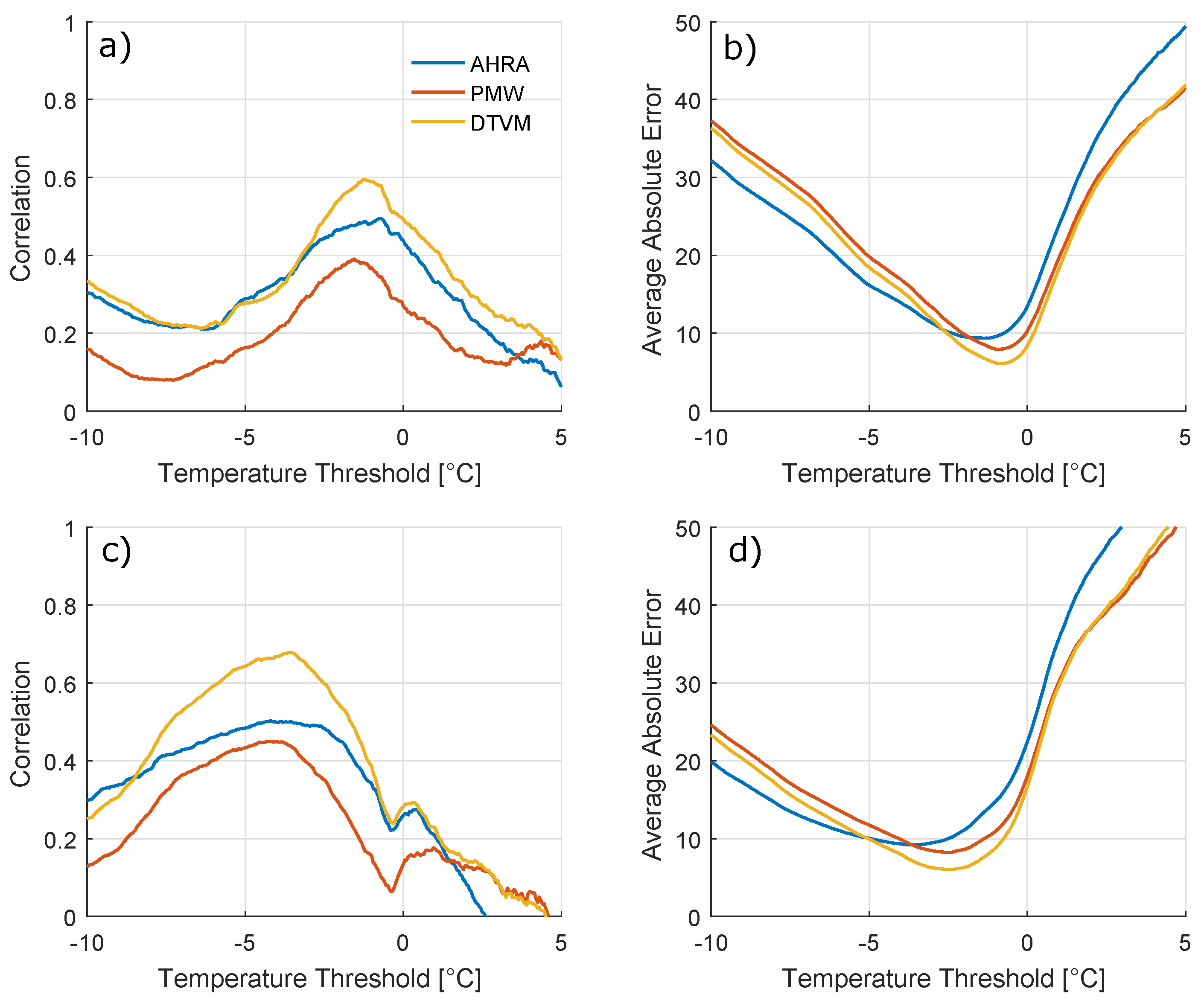
MO dates from AHRA, PMW and DTVM were compared to SAT derived MO dates using a spatial analysis. The average absolute difference and the correlation were calculated between each set of passive microwave MO dates and the SAT MO dates. This analysis was completed using a range of thresholds for the SAT data to determine the dependency of correlation and absolute difference on the SAT MO threshold values. Summary relationships for the 14-day average method and the daily average method are provided in Figure 6. It can be seen in Figure 6a,b that the correlation between MO from SAT and MO from DTVM is higher than than the correlation between MO from SAT and MO from the other two passive microwave MO methods over all temperatures of interest.The absolute differences are lower for DTVM when the temperature threshold is greater than approximately −2 C. Consistent results are found when a 14-day averaged SAT is used Figure 6c,d, indicating that the results are not due to the choice of SAT averaging window. While these results indicate that DTVM is in better agreement with a SAT-based MO method, we note that atmospheric indicators, such as air temperature and longwave radiation, can fluctuate above and below thresholds without necessarily a significant change in surface properties [1,2].
4.3. Comparison with Profiler Temperature Data
To assess the relative effectiveness of passive microwave MO methods, time series of snow/ice interface temperature and SAT (measured approximately 0.5 m above the snow/ice surface) collected from temperature profilers in the study region were compared with MO dates from DTVM. Data from six temperature profilers were available and all time series were examined. The profilers were located in regions of thick first-year ice as identified by the Canadian Ice Service weekly regional ice charts. Overall, the majority of the MO dates from the profiler data were in good agreement with that from DTVM. A representative time series is provided in Figure 7. It can be seen that the DTVM MO date agrees closely with a rise of surface temperature above freezing.
4.4. Dependence on Ice Type
In some cases, the MO date can be seen to change significantly over a short geographic distance. Such behaviour can also be seen in the AHRA and PWM algorithms, and suggests a possible dependence on ice type. Comparisons between the MO dates estimated from the DTVM for FYI- and MYI-dominant zones were made using TB37V pixel data extracted from land-fast ice in the M’Clintock Channel portion of the CAA as shown in Figure 8. FYI and MYI types make up approximately 100% of the ice cover in each respective zone. MYI is normally found in high concentration in this portion of the CAA due to its advection into the region from elsewhere during the summer period. FYI grows in situ with fall-freeze up, and due to the land-fast nature of the ice in this region, remains largely devoid of ridges and deformation features. The MO date for MYI is earlier than FYI by 15 days, consistent with a pattern generally observed in the MO dates as seen in Figure 4. As the DTVM is swath-based, this pattern indicates greater variance of MYI TB37V due to diurnal fluctuations in air temperature close to the surface during early melt compared to FYI. The presence of small amounts of liquid water in snow over the radiometrically cool MYI leads to an increase in TB37V associated with a reduction of penetration depth and absorption due to volume scattering from air bubbles in the upper ice layer, combined with increased emission of moisture [27]. The variance in the FYI time series, observed to increase later in the season compared to MYI, points to less emission sensitivity to melting conditions until there is a large enough moisture content in the snow cover [24]. However, we note that these details depend on the preconditioning of the snowpack at the given location. At other locations, it was also observed that MO may not be associated with an immediate change in variability, but instead was indicated by a monotonic decrease in brightness temperature. Such a decrease could occur in FYI when the snow pack starts to warm (temperature at the snow-ice interface greater than −5 C), which leads to changes in the brine volume and grain size at the basal layer of the snowpack [15]. The changes could be relatively slow and monotonic if the air temperature is relatively cool and/or it is early enough in the season that there is limited incoming shortwave radiation.
4.5. Melt Onset Trends
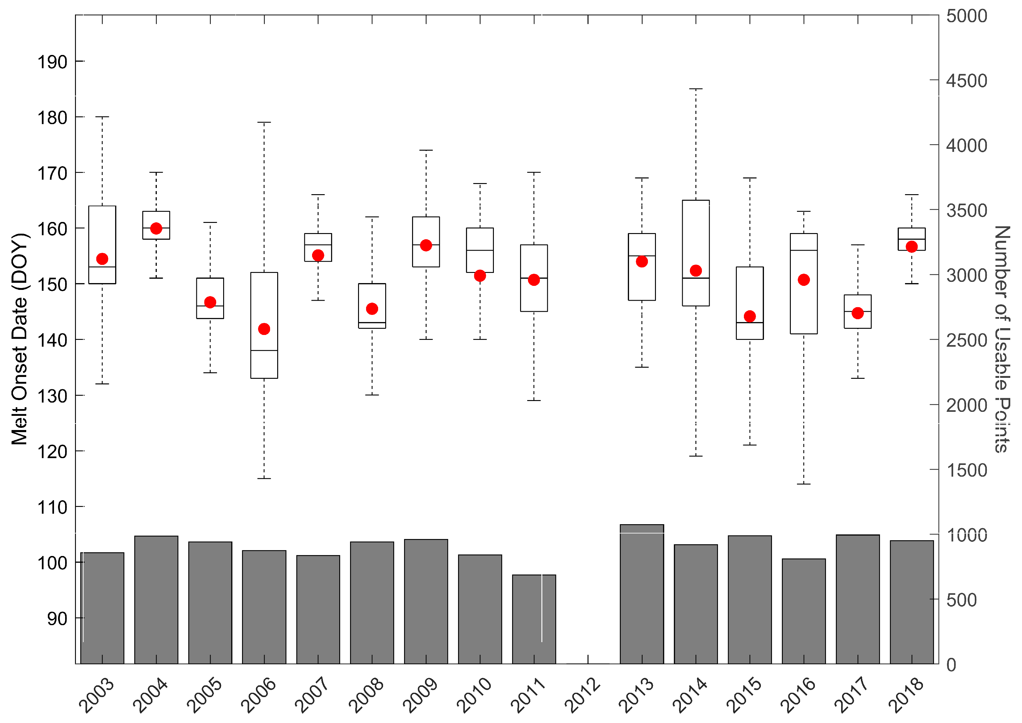
MO statistics; mean, median, 25 percentile and 75 percentile, were determined for each year AMSR data was available. This includes all years between 2003 and 2018, excluding 2012. The MO statistics were determined using all available MO dates determined for the 25 km grid within the CAA for each given year. The number of points for which MO was determined varied from year to year. Figure 9 provides a summary of the MO statistics as well as the number of points used. In some years, there may have been regions of the CAA for which the DTVM is not able to determine a MO date. This may have skewed the statistics provided in Figure 9. For example, if the majority of the missing points occur at a higher latitude for one year and then at a lower latitude for the next year, it may appear that the average MO occurs later the second year when they may actually occur at the same time. We do note that MO appears earlier in 2005 and 2006 in comparison to 2003, 2004 and 2007, which is consistent with results from [8].
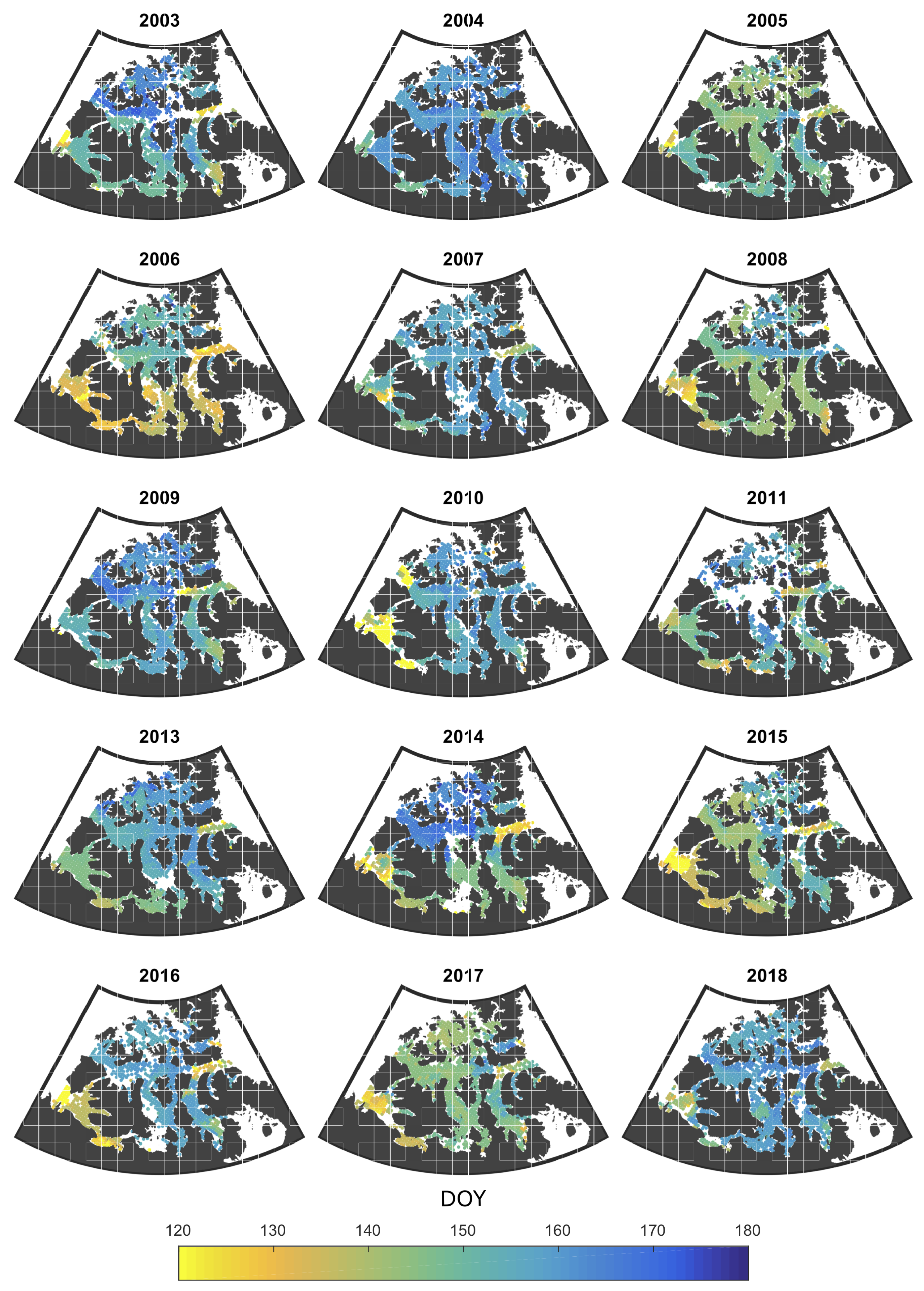
Similar to previous studies [9,28], a trend in mean MO dates is not observed. However, it can be seen that some years exhibit much larger range of MO dates than others. For example, 2004, 2007, 2017 and 2018 have a very narrow range of MO dates, while 2006, 2014, 2015 and 2016 all have a much wider range. From inspection of the spatial distribution of MO dates (Figure 10), it was found that the years with large ranges of MO dates also had a significant latitudinal dependence of MO dates. In these cases, the northern part of the CAA experienced melt 2–3 weeks later than the southern region. In contrast, for years with a narrow range of MO dates, the majority of the CAA experienced MO within approximately one week.
A preliminary investigation of the latitudinal dependence of MO was carried out through examination of Advanced Polar Pathfinder (APPx) data. APPx data have been used in earlier MO studies in the CAA [9,29] for trend analysis. We chose two years with very different MO patterns, 2006 and 2007, and averaged SAT and net longwave radiation at the surface for the month of May for each year. It was found the monthly average of net longwave radiation is higher in the southern part of the domain in 2006, whereas a latitudinal dependence is less obvious in 2007. In addition, SAT was lower in 2007 as compared to 2006. This has been noted in an earlier study [8], and is believed to have delayed MO in the CAA in 2007. These observations support the study by [30] in which a link was found between early MO and increased longwave downwelling radiation anomalies. A more thorough investigation of latitudinal dependence of MO will be investigated in a future study.
5. Discussion
Comparisons between MO dates estimated using three passive microwave methods, PMW, AHRA and DTVM, show that the modes of the differences are centred around 0. This indicates that, generally, the three passive microwave methods are in agreement. MO dates estimated using the DTVM and PMW methods agree more closely to each other than to the AHRA MO dates. This is likely a result of both the DTVM and PMW methods relying partly or entirely on the variability of TB37V. Both histograms in Figure 5, in which the AHRA is compared to the PMW and the DTVM, indicate bi-modal distributions centred around −1:1 and 8:10. This is strong evidence to suggest that, in the CAA, the 20-day window test, which is used by the AHRA, is estimating MO 9 days earlier than DTVM and PMW. The AHRA determined MO before a significant increase in surface temperature and before any significant change in the HR parameter. As the AHRA uses different channels it may be sensitive to different features of the surface signal. For example, horizontally polarized channels are known to be more sensitive to surface roughness than vertically polarized channels [31]. The HR parameter used in AHRA also has substantial overlapping signatures with wind-slab (due to blowing snow) and emission from a brine-rich snow layer [32], in particular during the range (−10 °C to 4 °C) that could trigger the 20 day window test.
To investigate the possibility that weather effects could be impacting MO dates, we examined the values of the polarization and gradient ratios that are used as weather filters in passive microwave ice concentration retrieval algorithms [19]. These ratios were generally found to stay below the thresholds that would indicate atmospheric effects, such as contamination of the surface signal by cloud liquid water or water vapour, hence, similar to previous studies, we believe 37 GHz can be used without correcting the brightness temperatures for atmospheric effects (at least in the landfast region considered here). However, this does not take into account the fact that increasing water vapour (and downwelling longwave radiation) can indirectly lead to changes in the snow cover and hence emissivity of the snowpack, which would then lead to changes in brightness temperature. This cannot be fully taken into account without a more detailed investigation. For example, by carrying out emission modelling (e.g., [33]). This is an exploratory area for current microwave emission models, and is outside the scope of the present study.
6. Conclusions
The dynamic threshold approach to MO (DTVM) provides an alternative to current passive microwave methods that improves upon the the spatial resolution and reduces the reliance of MO detection on fixed thresholds. It was found through comparison with SAT from reanalysis data and temperature profilers that the DTVM yields MO dates that are consistent with the SAT and surface temperature approaching the freezing point. At some locations in the study region, MO dates change significantly over a short distance. This is also seen in spatial maps of AHRA MO dates, and PMW MO dates, although for PMW it may be related to the algorithm design, which checks for spatial homogeneity of MO dates. Future work will include using microwave emission models to better understand the relationship between ice types and brightness temperatures during EMO, in addition to application of the method over a larger geographic region. For the latter investigation, it may be worthwhile to utilize the enhanced-resolution passive microwave data available from NSIDC, as this would require less time and storage in the data preparation phase.
Author Contributions
Conceptualization and methodology, S.M. and K.A.S. and R.K.S. Software, S.M. All authors contributed to preparing and revising the manuscript. Supervision, K.A.S., funding acquisition, R.K.S.
Funding
Funding for this research was provided by Polar Knowledge Canada (POLAR) grant #NST-1718-0024.
Acknowledgments
We would like to acknowledge passive microwave data provided by the National Snow and Ice Data Centre and the Japan Aerospace Exploration Agency. F The PMW data was extracted from the 1979–2018 melt onset update file as retrieved from ‘neptune.gsfc.nasa.gov’ on 30 October 2018.
Conflicts of Interest
The authors declare no conflict of interest.
References
- Else, B.; Papkyriakou, N.; Raddatz, R.; Galley, R.; Mundy, C.; Barber, D.; Swystun, K.; Rysgaard, S. Surface energy budget of landfast sea ice during the transitions from winter to snowmelt and melt pond onset: The importance of net longwave radiation and cyclone forcings. J. Geophys. Res. Ocean. 2014, 119, 3679–3693. [Google Scholar] [CrossRef]
- Persson, P.O.G. Onset and end of the summer melt season over sea ice: Thermal structure and surface energy perspective from SHEBA. Clim. Dyn. 2012, 39, 1349–1371. [Google Scholar] [CrossRef]
- Perovich, D.; Richter-Menge, J.; Jones, K.; Light, B.; Elder, B.; Polashenski, C.; Laroche, D.; Markus, T.; Lindsay, R. Arctic sea-ice melt in 2008 and the role of solar heating. Ann. Glaciol. 2011, 52, 355–359. [Google Scholar] [CrossRef] [Green Version]
- Vivier, F.; Hutchings, J.; Kawaguchi, Y.; Kikuchi, T.; Morison, J.; Lourenco, A.; Noguchi, T. Sea ice melt onset associated with lead opening during the spring/summer transition near the North Pole. J. Geophys. Res. 2016, 121, 2499–2522. [Google Scholar] [CrossRef] [Green Version]
- Perovich, D.; Light, B.; Eicken, H.; Jones, K.; Runciman, K.; Nghiem, S. Increasing solar heating of the Arctic Ocean and adjacent seas, 1979–2005: Attribution and role in the ice-albedo feedback. Geophys. Res. Lett. 2007, 34, L19505. [Google Scholar] [CrossRef]
- Petty, A.; Schröder, D.; Stroeve, J.; Markus, T.; Miller, J.; Kurtz, N.; Feltham, D.; Flocco, D. Skillful spring forecasts of September Arctic sea ice extent using passive microwave sea ice observations. Earth’s Future 2017, 5, 254–263. [Google Scholar] [CrossRef]
- Markus, T.; Stroeve, J.; Miller, J. Recent changes in Arctic sea ice melt onset, freezeup, and melt season length. J. Geophys. Res. 2009, 114, C12024. [Google Scholar] [CrossRef]
- Howell, S.E.; Tivy, A.; Yackel, J.J.; Else, B.G.; Duguay, C.R. Changing sea ice melt parameters in the Canadian Arctic Archipelago: Implications for the future presence of multiyear ice. J. Geophys. Res. Ocean. 2008, 113, 1–21. [Google Scholar] [CrossRef]
- Mahmud, M.; Howell, S.; Geldsetzer, T.; Yackel, J. Detection of melt onset over the northern Canadian Arctic Archipelago sea ice from RADARSAT, 1997–2014. Remote. Sens. Environ. 2016, 178, 59–69. [Google Scholar] [CrossRef]
- Mortin, J.; Howell, S.; Wang, L.; Derksen, C.; Svensson, G.; Graversen, R.; Schroder, T. Extending the QuikSCAT record of seasonal melt-freeze transitions over Arctic sea ice using ASCAT. Remote. Sens. Environ. 2014, 141, 214–230. [Google Scholar] [CrossRef]
- Mortin, J.; Schroder, M.; Hansen, A.; Holt, B.; McDonald, K. Mapping of seasonal freeze-thaw transitions across the pan-Arctic land and sea ice domains with satellite radar. J. Geophys. Res. Ocean. 2012, 117, C08004. [Google Scholar] [CrossRef]
- Bliss, A.C.; Anderson, M.R. Arctic Sea Ice Melt Onset Timing From Passive Microwave-Based and Surface Air Temperature-Based Methods. J. Geophys. Res. Atmos. 2018, 123, 9063–9080. [Google Scholar] [CrossRef]
- Drobot, S.; Anderson, M. An improved method for determining snowmelt onset dates over Arctic sea ice using scanning multichannel microwave radiometer and special sensor microwave/imager data. J. Geophys. Res. 2001, 106, 24033–24049. [Google Scholar] [CrossRef]
- Tedesco, M. Snowmelt detection over the Greenland ice sheet from SSM/I brightness temperature daily variations. Geophys. Res. Lett. 2007, 34. [Google Scholar] [CrossRef] [Green Version]
- Barber, D. Microwave remote sensing, sea ice and arctic climate. Phys. Can. 2005, 8, 105–111. [Google Scholar]
- Livingstone, C.; Singh, K.; Gray, A. Seasonal and regional variations of active/passive microwave signatures of sea ice. IEEE Trans. Geosci. Remote. Sens. 1987, GE-25, 159–173. [Google Scholar] [CrossRef]
- Lavergne, T.; Sorensen, A.; Kern, S.; Tonboe, R.; Notz, D.; Signe, A.; Bell, L.; Dybkjaer, G.; Eastwood, S.; Gabarro, C.; et al. Version 2 of the EUMETSAT OSI SAF and ESA CCI sea ice concentration climate data records. Cryosphere 2019, 13, 49–78. [Google Scholar] [CrossRef]
- Bromwich, D.H.; Wilson, A.B.; Bai, L.S.; Moore, W.K.; Bauer, P. A comparison of the regional Arctic System Reanalysis and the global ERA-Interim Reanalysis for the Arctic. Q. J. R. Meteorol. Soc. 2016, 142, 644–658. [Google Scholar] [CrossRef]
- Spreen, G.; Kaleschke, L.; Heybster, G. Sea ice remote sensing using AMSR-E 89 GHz channels. J. Geophys. Res. 2008, 113, C02303. [Google Scholar] [CrossRef]
- Paynter, C. Oceanetic 908 Drifter Buoy Sensor Description. 2014. Available online: https://wiki.oceannetworks.ca/download/attachments/38076681/Oceanetic+908+Drifter+Buoy+Sensor+Description.pdf (accessed on 20 December 2018).
- Bliss, A.C.; Miller, J.A.; Meier, W.N. Comparison of passive microwave-derived early melt onset records on Arctic sea ice. Remote. Sens. 2017, 9, 199. [Google Scholar] [CrossRef]
- Bliss, A.C.; Anderson, M.R. Snowmelt onset over Arctic sea ice from passive microwave satellite data: 1979–2012. Cryosphere 2014, 8, 2089–2100. [Google Scholar] [CrossRef]
- Smith, M. Observation of perennial Arctic sea ice melt and freeze-up using passive microwave data. J. Geophys. Res. 1998, 103, 27753–27769. [Google Scholar] [CrossRef]
- Harouche, I.P.F.; Barber, D.G. Seasonal charcaterization of microwave emissions from snow-covered first-year sea ice. Hydrol. Process. 2001, 15, 3571–3583. [Google Scholar] [CrossRef]
- Rigor, I.; Colony, R.; Martin, S. Variations in surface air temperature observations in the Arctic, 1979-97. J. Clim. 2000, 13, 896–914. [Google Scholar] [CrossRef]
- Wang, L.; Derksen, C.; Brown, R.; Markus, T.; Peng, G.; Steele, M.; Bliss, A.; Meier, W.; Dickinson, S. Recent changes in pan-Arctic melt onset from satellite passive microwave measurements. Remote Sens. 2013, 10, 522–528. [Google Scholar] [CrossRef]
- Belchansky, G.; Douglas, D.; Mordvintsev, L.; Platnov, N. Estimating the time of melt onset and freeze onset over Arctic sea ice area using active and passive microwave data. Remote Sens. Environ. 2004, 92, 21–39. [Google Scholar] [CrossRef]
- Stroeve, J.; Markus, T.; Boisvert, L.; Miller, J.; Barrett, A. Changes in Arctic melt season and implications for sea ice loss. Geophys. Res. Lett. 2014, 41, 1216–1225. [Google Scholar] [CrossRef]
- Mulit-year sea-ice conditions in the western Canadian Arctic Archipelago region of the Northwest Passage: 1968–2008. Atmos. Ocean. 2008, 46, 229–242. [CrossRef]
- Mortin, J.; Svensson, G.; Graversen, R.G.; Kapsch, M.L.; Stroeve, J.C.; Boisvert, L.N. Melt onset over Arctic sea ice controlled by atmospheric moisture transport. Geophys. Res. Lett. 2016, 43, 6636–6642. [Google Scholar] [CrossRef] [Green Version]
- Stroeve, J.; Markus, T.; Maslanik, J.; Cavalieri, D.; Gasiewski, A.; Heinrichs, J.; Holmgren, J.; Perovich, D.; Sturm, M. Impact of surface roughness on AMSR-E sea ice products. IEEE Trans. Geosci. Remote Sens. 2006, 44, 3103–3117. [Google Scholar] [CrossRef]
- Hwang, B.; Langlois, A.; Barber, D.; Papakyrakou, T. On detection of the thermophysical state of landfast first-year sea ice using in-situ microwave emission during spring melt. Remote Sens. Environ. 2007, 111, 148–159. [Google Scholar] [CrossRef]
- Willmes, S.; Nicolaus, M.; Haas, C. The microwave emissivity variability of snow covered first-year sea ice from late winter to early summer: a model study. Cryosphere 2014, 8, 891–904. [Google Scholar] [CrossRef] [Green Version]
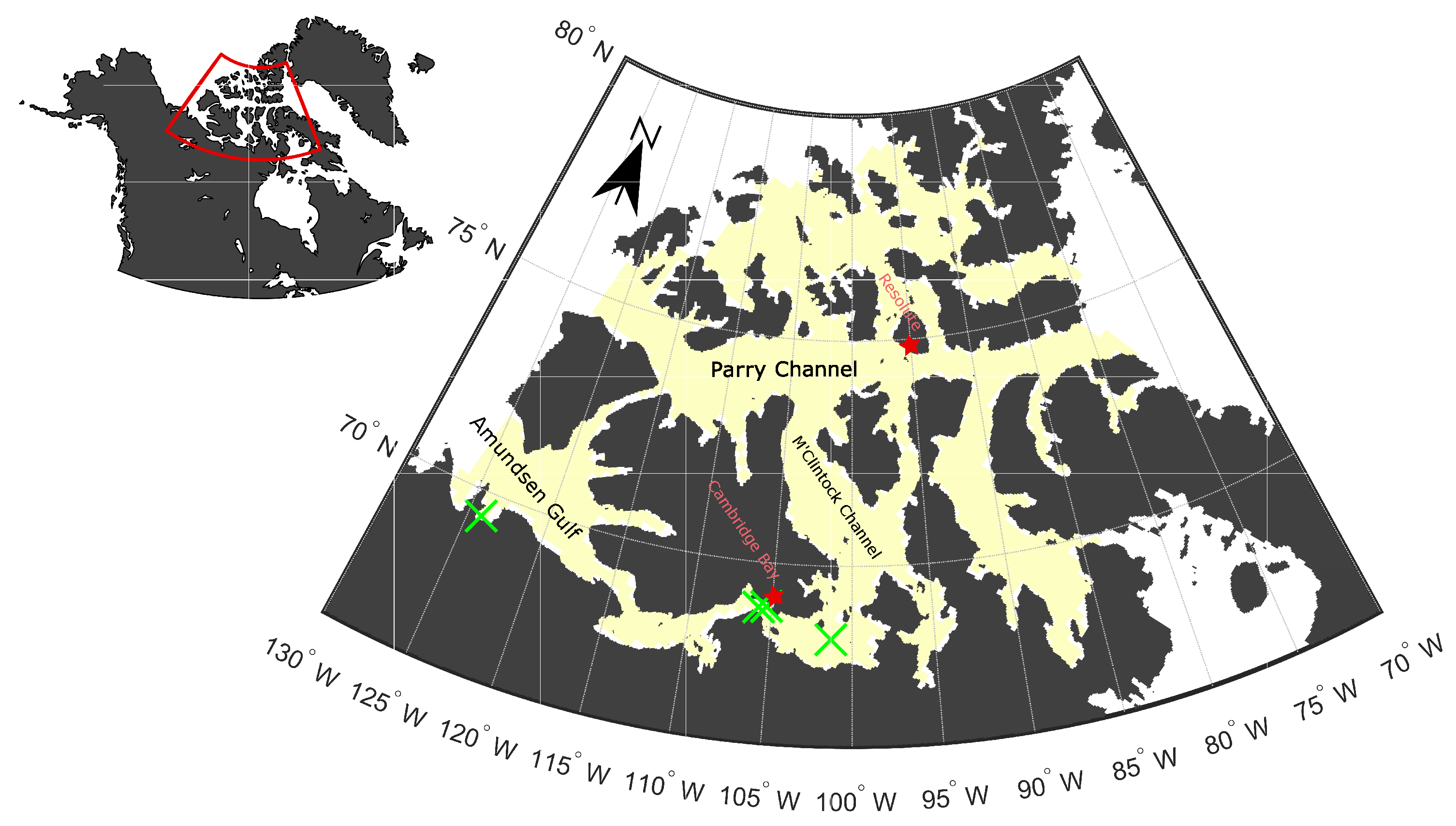
Figure 1.
The National Snow and Ice Data Center (NSIDC) region definition of the Canadian Arctic Archipelago (CAA) (light yellow). The locations of the profiler data used for validation are indicated by the green markers. The blue box indicates the approximate location of the Sentinel-1 image used in the discussion of melt onset (MO) for first year and multiyear ice (Section 5).

Figure 2.
Data from pixel at [69.87°N, −88.15°W], 2017. (a) Time series of the variability of TB37V over the entire year (black). A series of thresholds (green) and their corresponding MO dates (blue). (b) A histogram of MO dates corresponding to 500 potential threshold values. Blue bars represent values found within the melt range and grey bars represent values outside. The red line represents the 25th percentile of the accepted data which is then defined as the MO date and the red region represents the interquartile range (IQR).

Figure 3.
Data from pixel at [69.87°N, −88.15°W], 2017. (a) Swath-to-swath TB37V data (black) and daily averaged TB37V data (green). (b) Standard deviation of swath data (black) and standard deviation of daily averaged data (green). The vertical red line indicates the MO date using swath-to-swath data and the Dynamic Threshold Variability Method (DTVM). The vertical blue line indicates the MO date using daily averaged data and the DTVM.

Figure 4.
MO dates in the CAA for 2003. (a) AHRA 25 km grid, (b) PMW 25 km grid, (c) DTVM 25 km grid, (d) DTVM 6 km Grid.
Figure 4.
MO dates in the CAA for 2003. (a) AHRA 25 km grid, (b) PMW 25 km grid, (c) DTVM 25 km grid, (d) DTVM 6 km Grid.

Figure 5.
Normalized histogram of MO date differences by pixel for years from 2003 to 2011 (a) DTVM-AHRA, (b) DTVM-PMW, (c) PMW-AHRA.
Figure 5.
Normalized histogram of MO date differences by pixel for years from 2003 to 2011 (a) DTVM-AHRA, (b) DTVM-PMW, (c) PMW-AHRA.

Figure 6.
(a) Correlation between MO dates derived from daily averaged SAT values for various SAT thresholds (b) Absolute difference between MO dates derived from daily averaged SAT values for various SAT thresholds (c) Correlation between MO dates derived from 14-day averaged SAT values at various thresholds (d) Absolute difference between MOs derived from 14-day averaged SAT values at various thresholds. Statistics were calculated using data points for which all three methods had a MO data from year 2003 to 2011 (6147 points in total).

Figure 7.
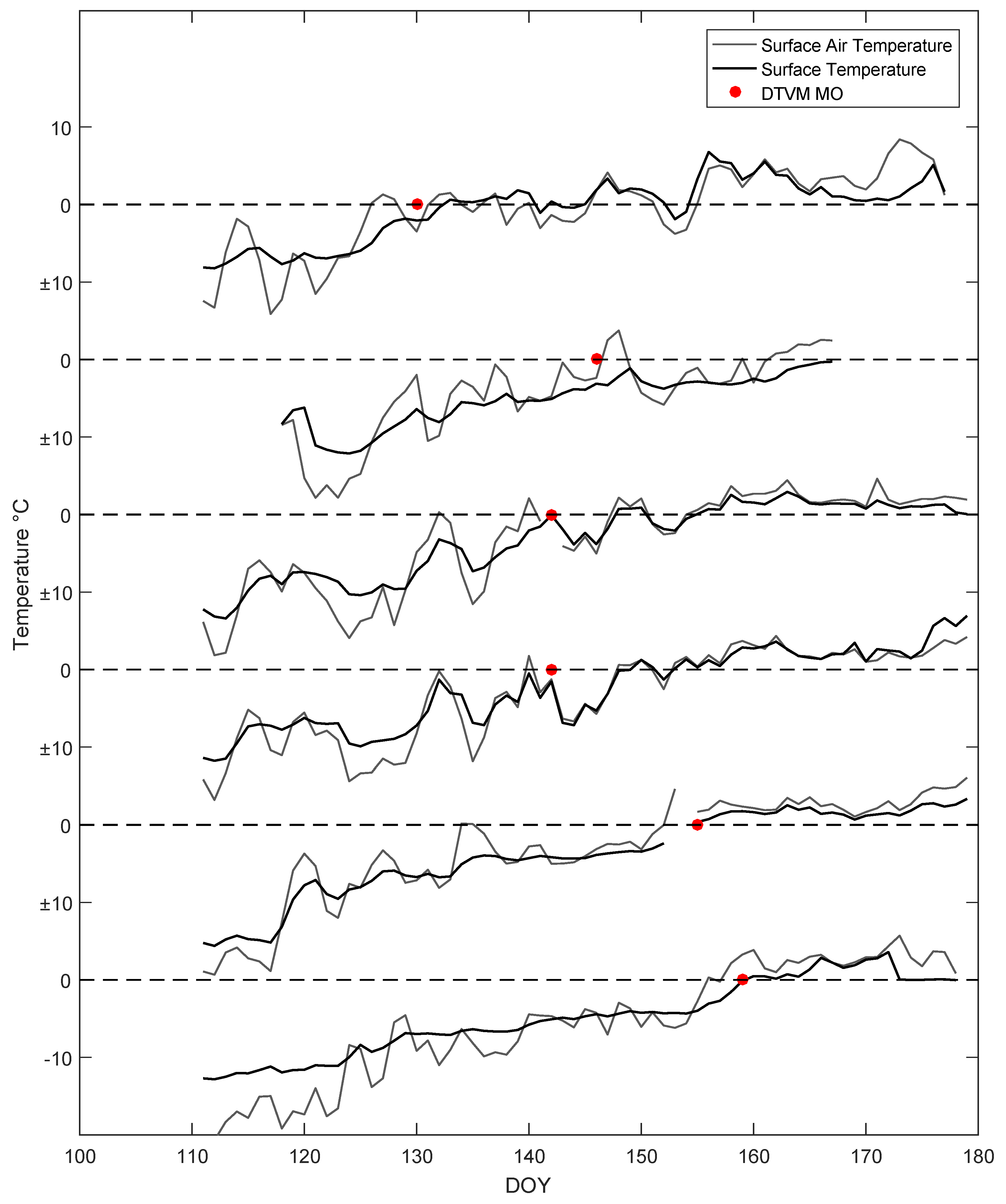
Snow/ice interface temperature and SAT from profilers located in the study region (locations shown in Figure 1) with MO dates from DTVM indicated. Order is profile 1–6 from top to bottom: same orientation as in Table 2.

Figure 8.
(a) Location of first-year sea ice (FYI) and multiyear ice (MYI) pixels sampled in the CAA in 2018, shown on a Sentinel-1 synthetic aperture radar image acquired on Day 126, in the late-winter period prior to MO. (b) Time series of 37V brightness temperature of FYI. (c) Time series of DTVM applied to FYI, with vertical bar denoting MO on Day 164. (d) Time series of 37 V brightness temperature of MYI. (e) Time series of DTVM applied to MYI, with vertical bar denoting MO on Day 149.

Figure 9.
DTVM MO statistics from 2003 to 2018 at the 25 km resolution. Red dots indicate mean MO value for each year. Horizontal lines indicate the median and box edges indicate the 25 and 75 percentiles. Maximum and minimum values indicate the maximum and minimum values from each year not considered an outlier. Outliers are defined as points farther than three scaled median absolute deviations from the median. The bar chart at the base of the figure indicates the number of points used for each year to determine the statistics.

Figure 10.
DTVM MO dates for the CAA from 2003 to 2018 at 25 km resolution.


Table 1.
Comparison between MO dates (in days) for the passive microwave MO methods used in this study.
Table 1.
Comparison between MO dates (in days) for the passive microwave MO methods used in this study.
| Mode | Mean | Standard Deviation | |
|---|---|---|---|
| DTVM-AHRA | 0 | 5.35 | 14.59 |
| DTVM-PMW | 2 | 0.52 | 12.50 |
| PMW-AHRA | 0 | 4.84 | 17.81 |
Table 2.
Location and DTVM MO dates for temperature profilers in the study region.
| Instrument | Ice Type | Latitude | Longitude | Year | DTVM MO |
|---|---|---|---|---|---|
| profiler 1 | FYI | 69.44N | 124.1W | 2014 | 130 |
| profiler 2 | FYI | 69.03N | 105.3W | 2014 | 146 |
| profiler 3 | FYI | 69.00N | 105.8W | 2015 | 141 |
| profiler 4 | FYI | 68.37N | 101.3W | 2015 | 142 |
| profiler 5 | FYI | 69.00N | 105.8W | 2016 | 155 |
| profiler 6 | FYI | 68.88N | 105.8W | 2018 | 158 |
© 2019 by the authors. Licensee MDPI, Basel, Switzerland. This article is an open access article distributed under the terms and conditions of the Creative Commons Attribution (CC BY) license (http://creativecommons.org/licenses/by/4.0/).
Share and Cite
MDPI and ACS Style
Marshall, S.; Scott, K.A.; Scharien, R.K. Passive Microwave Melt Onset Retrieval Based on a Variable Threshold: Assessment in the Canadian Arctic Archipelago. Remote Sens. 2019, 11, 1304. https://doi.org/10.3390/rs11111304
AMA Style
Marshall S, Scott KA, Scharien RK. Passive Microwave Melt Onset Retrieval Based on a Variable Threshold: Assessment in the Canadian Arctic Archipelago. Remote Sensing. 2019; 11(11):1304. https://doi.org/10.3390/rs11111304
Chicago/Turabian StyleMarshall, Stephen, K. Andrea Scott, and Randall K. Scharien. 2019. "Passive Microwave Melt Onset Retrieval Based on a Variable Threshold: Assessment in the Canadian Arctic Archipelago" Remote Sensing 11, no. 11: 1304. https://doi.org/10.3390/rs11111304
Note that from the first issue of 2016, this journal uses article numbers instead of page numbers. See further details here.