Introduction
This tutorial is a supplement to our tutorial on indexing candidate pairs with the recordlinkage Python package for data integration. This tutorial takes a closer look at the sorted neighbourhood indexing method, which has more complex behaviour than other indexing methods. To get the most out of this tutorial, you should already be familiar with indexing candidate pairs with recordlinkage.
This tutorial contains a series of examples, which are intended to demonstrate both the power and the quirks of the sorted neighbourhood method.
The interleaved neighbourhood
Consider the following code, which creates a set of candidate links using the sorted neighbourhood method:
import pandas as pd

import recordlinkage as rl


# Name data for indexing

names_1 = ['alfred', 'bob', 'calvin', 'hobbes', 'rusty']

names_2 = ['alfred', 'danny', 'callum', 'hobie', 'rusty']


# Convert to DataFrames

df_a = pd.DataFrame(pd.Series(names_1, name='names'))

df_b = pd.DataFrame(pd.Series(names_2, name='names'))


# Create indexing object

indexer = rl.SortedNeighbourhoodIndex(on='names', window=3)


# Create pandas MultiIndex containing candidate links

candidate_links = indexer.index(df_a, df_b)
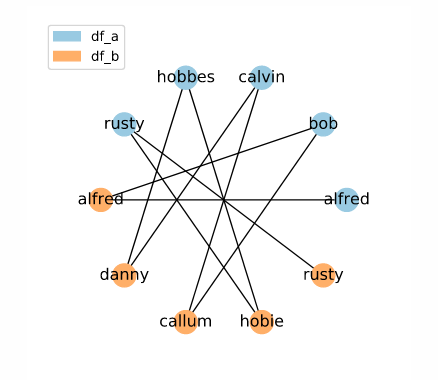
As can be seen in the network diagram of the result, we have candidate links between all names which would be adjacent in a sorted list. This shows how the sorted neighbourhood method can be used to identify candidate links even when you cannot guarantee exact matches between potential matches. However, knowing how this is processed internally is important for understanding when this method might return unexpected results.
Internally, the SortedNeighbourhoodIndex does the following to determine candidate links:
- It places the data from both data frames into one series.
- It sorts the series.
- For each element, it looks within the specified
window. If two elements from different data frames are within the window, they are considered a candidate link.
Let’s look at this process step-by-step. First, we start with two sets of names:
names_1 = ['alfred', 'bob', 'calvin', 'hobbes', 'rusty']

names_2 = ['alfred', 'danny', 'callum', 'hobie', 'rusty']
These are combined into a single sorted series (seen here as a sorted list):
['alfred', 'alfred', 'bob', 'callum', 'calvin', 'danny', 'hobbes', 'hobie', 'rusty', 'rusty']
Since window = 3, the SortedNeighbourhoodIndex finds candidate links for each element by looking at three elements total, centred on the element in question. In other words, a window of 3 means that only elements that are adjacent to the target (i.e. one position away) are considered as candidate links.
To visualize this, let’s look at a few windows in the list by capitalizing entries inside the window. The window for the first 'alfred' looks like this:
[ALFRED, ALFRED, 'bob', 'callum', 'calvin', 'danny', 'hobbes', 'hobie', 'rusty', 'rusty']
Since each 'alfred' is from a different data frame, a candidate link is given, as can be seen in the network above. The next window, centered on the second 'alfred', looks like this:
[ALFRED, ALFRED, BOB, 'callum', 'calvin', 'danny', 'hobbes', 'hobie', 'rusty', 'rusty']
And since the second 'alfred' is from a different data frame than 'bob', another candidate link is created. The process continues:
['alfred', ALFRED, BOB, CALLUM, 'calvin', 'danny', 'hobbes', 'hobie', 'rusty', 'rusty']

['alfred', 'alfred', BOB, CALLUM, CALVIN, 'danny', 'hobbes', 'hobie', 'rusty', 'rusty']

['alfred', 'alfred', 'bob', CALLUM, CALVIN, DANNY, 'hobbes', 'hobie', 'rusty', 'rusty']

['alfred', 'alfred', 'bob', 'callum', CALVIN, DANNY, HOBBES, 'hobie', 'rusty', 'rusty']

['alfred', 'alfred', 'bob', 'callum', 'calvin', DANNY, HOBBES, HOBIE, 'rusty', 'rusty']

['alfred', 'alfred', 'bob', 'callum', 'calvin', 'danny', HOBBES, HOBIE, RUSTY, 'rusty']

['alfred', 'alfred', 'bob', 'callum', 'calvin', 'danny', 'hobbes', HOBIE, RUSTY, RUSTY]

['alfred', 'alfred', 'bob', 'callum', 'calvin', 'danny', 'hobbes', 'hobie', RUSTY, RUSTY]
As we can see in the network visualization above, this process yields two candidate links for every entry, except for the first and last. However, it is important to note that this data is extremely unusual, and only occurs because the elements of each data frame alternate consistently in the sorted series. We can see this if we capitalize all the elements from df_a:
[ALFRED, 'alfred', BOB, 'callum', CALVIN, 'danny', HOBBES, 'hobie', RUSTY, 'rusty']
With different name data, we will see that individual records may be given significantly more, or significantly fewer, candidate links depending on biases in the input data.
The small neighbourhood
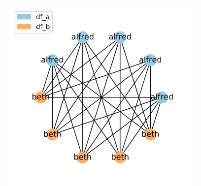
What if the sorted neighbourhood contains very few unique elements? Here, we can see the sorted list that would occur if df_a contained only alfred and df_b contained only beth.
[ALFRED, ALFRED, ALFRED, ALFRED, ALFRED, 'beth', 'beth', 'beth', 'beth', 'beth']
Since alfred and beth are contained in the same window (i.e. are adjacent), all cases of alfred and beth are considered adjacent. The resulting set of candidate links is equivalent to what would be created with the Full Index method:
The divided neighbourhood
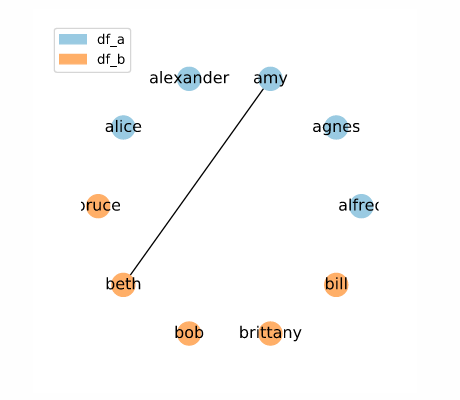
On the other hand, consider another case where the all elements from df_a are sorted before the elements of df_b, but each name is a distinct value:
[AGNES, ALEXANDER, ALFRED, ALICE, AMY, 'beth', 'bill', 'bob', 'brittany', 'bruce']
Here, only a single link is created! This is because only a single pair of elements from different data frames appear within the same window ('alice' and 'beth').
The random neighbourhood
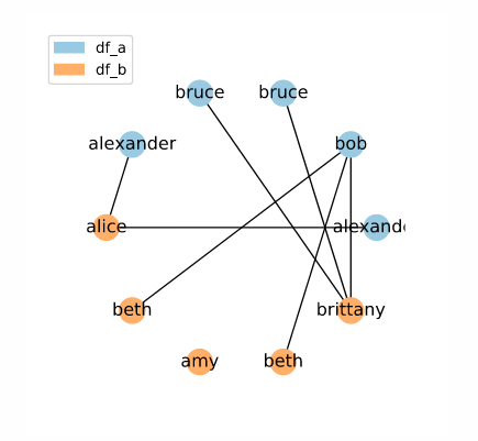
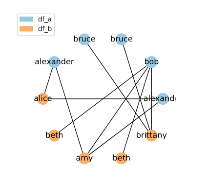
Just like our original test data showed unusually predictable behaviour, the small neighbourhood and divided neighbourhood examples are extreme cases which highlight the idiosyncrasies of the sorted neighbourhood method. To get a better sense of how sorted neighbour indexing will perform in the real world, let’s look at a random selection of these names:
[ALEXANDER, ALEXANDER, 'alice', 'amy', 'beth', 'beth', BOB, 'brittany', BRUCE, BRUCE]
Here, our randomly selected names un unevenly interspersed, and so we get a less regular pattern.
Choosing a window size
All of these examples maintain the default window size of 3. However, you may find it useful to widen the window. Widening the window will cause a greater number of candidate links to be included. For example, this is what our random neighbourhood example looks like with the window size increased to 5:
While a larger set of candidate keys will require more computational resources to compare, a larger set may be worth the decreased efficiency. A larger window is less susceptible to idiosyncratic orderings, and will reduce the chance of excluding a true match during the indexing phase. It is important to remember that the goal of indexing is not to find final matches — it is to discard obvious mismatches.
Summary
The sorted neighbourhood indexing method is a great tool for increasing efficiency in record linkage, even when exact match blocking is not possible. However, this method has some unusual behaviour that, with unusual data, may create significantly more or significantly fewer candidate links than expected. The sorted neighbourhood method will perform best when there are no systematic differences in the input data, which could cause unexpected behaviour when the data is combined and sorted.