Welcome to the second installment of a five part tutorial series on the recordlinkage Python package. Each tutorial will cover a specific stage of the data integration workflow. The topics and links for each tutorial are included below:
- Pre-processing with recordlinkage
- Indexing candidate links with recordlinkage
- Record comparison with recordlinkage
- Record pair classification with recordlinkage
- Data fusion (coming soon …)
What is data indexing?
When using recordlinkage for data integration or deduplication, indexing is the process of identifying pairs of data frame rows which might refer to the same real-world entity. These matched rows are known as candidate links. The goal of the indexing stage of data integration is to exclude obvious non-matches from the beginning of your analysis to improve computational efficiency.
The easiest, but least efficient, indexing method is to consider every possible link as a candidate link. Using this method for integrating two data frames, we would be comparing every row in the first data frame with every row in the second. So, if we had ten rows in the first data frame and five in the second, we would be considering 50 (10 × 5) candidate links. This growth in complexity can be visualized simply by drawing a 10 × 5 rectangle where coloured squares indicate candidate links:
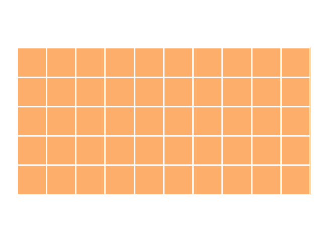
As you can see, every possible link is coloured. With such a large set of candidate links, every comparison made between the two data frames must be made length(DataFrame A) × length(DataFrame B) times. This isn’t a problem with only 50 candidate links. However, most data integration problems are much larger. If we instead had 10,000 records in data frame A and 100,000 records in data frame B, we would have 1,000,000,000 candidate links. In the world of big data, 100,000 records barely qualifies as “medium-sized data” — and yet, our data integration problem has become large enough to be difficult on consumer laptops. Luckily, there’s a better way.
In most data integration problems, the majority of possible links will be non-matches, and so we want to use our knowledge of the data we’re integrating to eliminate bad links from the outset.
Let’s consider an imaginary example in which we are integrating two datasets of employee information. Supposing that we have accurate “city of residence” data for all employees, and assuming that each employee lives in only one city, we can rule out links between rows with mismatching cities. Like before, we can visualize what this might look like if employees lived in three cities, where coloured blocks represent candidate links (see how these graphics were generated):
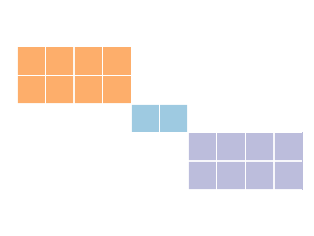
This indexing method is known as “blocking”. By blocking on city, we were able to reduce our set of candidate links from 50 links to 18 links, or 36% of all possible links. In our earlier example with larger datasets, this magnitude in reduction would reduce the number of candidate links from 1,000,000,000 to 360,000,000. However, we’re likely to get even greater reductions if we use blocking variables with more categories, or were blocking on multiple variables. For example, by blocking on given_name in the febrl4 example datasets included with recordlinkage, we can reduce the set of candidate links from 25,000,000 (5000 × 5000) to a mere 77,249 (0.3% of all possible links).
However, keep in mind that fewer candidate links are not always better, since you don’t want to throw away actual matches. The ideal indexing strategy will discard a large number of mismatching records but discard very few matching records. It is important to have a deep understanding of your data, and the indexing methods that you apply to it, to ensure that you do not erroneously discard matching records.
Indexation methods
This table is a straight-up information dump, which overviews all of the indexing methods built-in to recordlinkage:
| Method | Description | Advantages | Limitations | |
|---|---|---|---|---|
| 0 | Full Index | All possible links are kept as candidate links. | Convenient when performance isn't an issue. | Highly inefficient with large data sets. |
| 1 | Block Index | Only links exactly equal on specified values are kept as candidate links. | Extremely effective for high-quality, structured data. | Does not allow approximate matching. |
| 2 | Sorted Neighbourhood Index | Rows are ranked by some value, and candidate links are made between rows with nearby values. | Useful for making approximate matches. | More conceptually difficult. |
| 3 | Random Index | Creates a random set of candidate links. | Useful for developing your data integration workflow on a subset of candidate links, or creating training data for unsupervised learning models. | Not recommended for your final data integration workflow. |
Code examples and visualizations
We will now demonstrate how to use each indexing method in recordlinkage, and visualize the resulting set of candidate links.
The indexing process has two simple steps:
- Create an
Indexobject to manage the indexing process. We call this theindexerin the following code examples. - Call
indexer.index()to return a PandasMultiIndexobject. This object identifies candidate links by their original indices in the data frames being linked.
Once you have created the MultiIndex, you can use these candidate links to begin the record comparison stage of the data integration process.
Setup
We’ll demonstrate these indexing algorithms by indexing candidate links between two lists of names. To start, we need to add this data to two Pandas data frames.
import pandas as pd

import recordlinkage as rl


# Name data for indexing

names_1 = ['alfred', 'bob', 'calvin', 'hobbes', 'rusty']

names_2 = ['alfred', 'danny', 'callum', 'hobie', 'rusty']


# Convert to DataFrames

df_a = pd.DataFrame(pd.Series(names_1, name='names'))

df_b = pd.DataFrame(pd.Series(names_2, name='names'))
Full index
The following code creates a set of candidate links using the full index method:
# Create indexing object

indexer = rl.FullIndex()


# Create pandas MultiIndex containing candidate links

candidate_links = indexer.index(df_a, df_b)
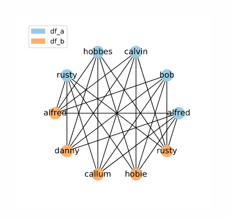
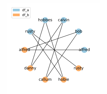
The result is a set of candidate links containing all possible links. The image above visualizes the set of candidate links as a network, with data frame rows as labelled nodes and candidate links as connections between them. You can also click the button to see the candidate links by their original indices (i.e. the contents of the MultiIndex containing the candidate links).
Blocked index
The following code creates a set of candidate links using the block index method:
# Create indexing object

indexer = rl.BlockIndex(on='names')


# Create pandas MultiIndex containing candidate links

candidate_links = indexer.index(df_a, df_b)
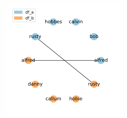
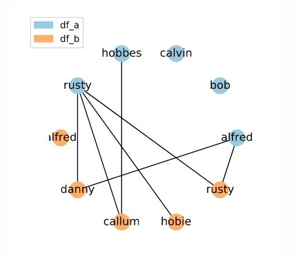
Here, the set of candidate links is restricted to entries with the exact same name. Think carefully about the quality of your data when using this method. If you cannot guarantee exact matches between corresponding rows, you may exclude potential matches from your set of candidate links.
Random index
The following code creates a set of candidate links using the random index method:
# Create indexing object

indexer = rl.RandomIndex()


# Create pandas MultiIndex containing candidate links

candidate_links = indexer.index(df_a, df_b)
Here, we have a random set of candidate links.
Sorted neighbourhood index
The sorted neighbourhood method is more complex than other indexing methods. The following code creates a set of candidate links using the sorted neighbourhood index method:
# Create indexing object

indexer = rl.SortedNeighbourhoodIndex(on='names', window=3)


# Create pandas MultiIndex containing candidate links

candidate_links = indexer.index(df_a, df_b)
Here, we have candidate links between names which would be adjacent in a sorted list. This method is excellent if you want to reduce the number of candidate links considered, but cannot guarantee exact matches between potential matches. However, it’s important to understand that this method has some quirks which should be kept in mind while using it. To learn more about sorted neighbourhood indexing check out our deep dive tutorial.
What's next?
After you have created a set of candidate links, you’re ready to begin comparing the records associated with each candidate link. The next step will look like this:
᠁

# Create pandas MultiIndex containing candidate links

candidate_links = indexer.index(df_a, df_b)


# Create comparing object

comp = rl.Compare(candidate_links, df_a, df_b)
For an introduction to record comparison, check out the next tutorial in this series, record comparison with recordlinkage.
Further reading
We highly recommend that you check out the recordlinkage documentation section on indexing. For an in-depth look at the mechanics of each indexing class, check out the indexing page of the recordlinkage API Reference.