Kelvin-Helmholtz and Holmboe instability
Please click on a picture for the animation.
Kelvin Helmholtz instability
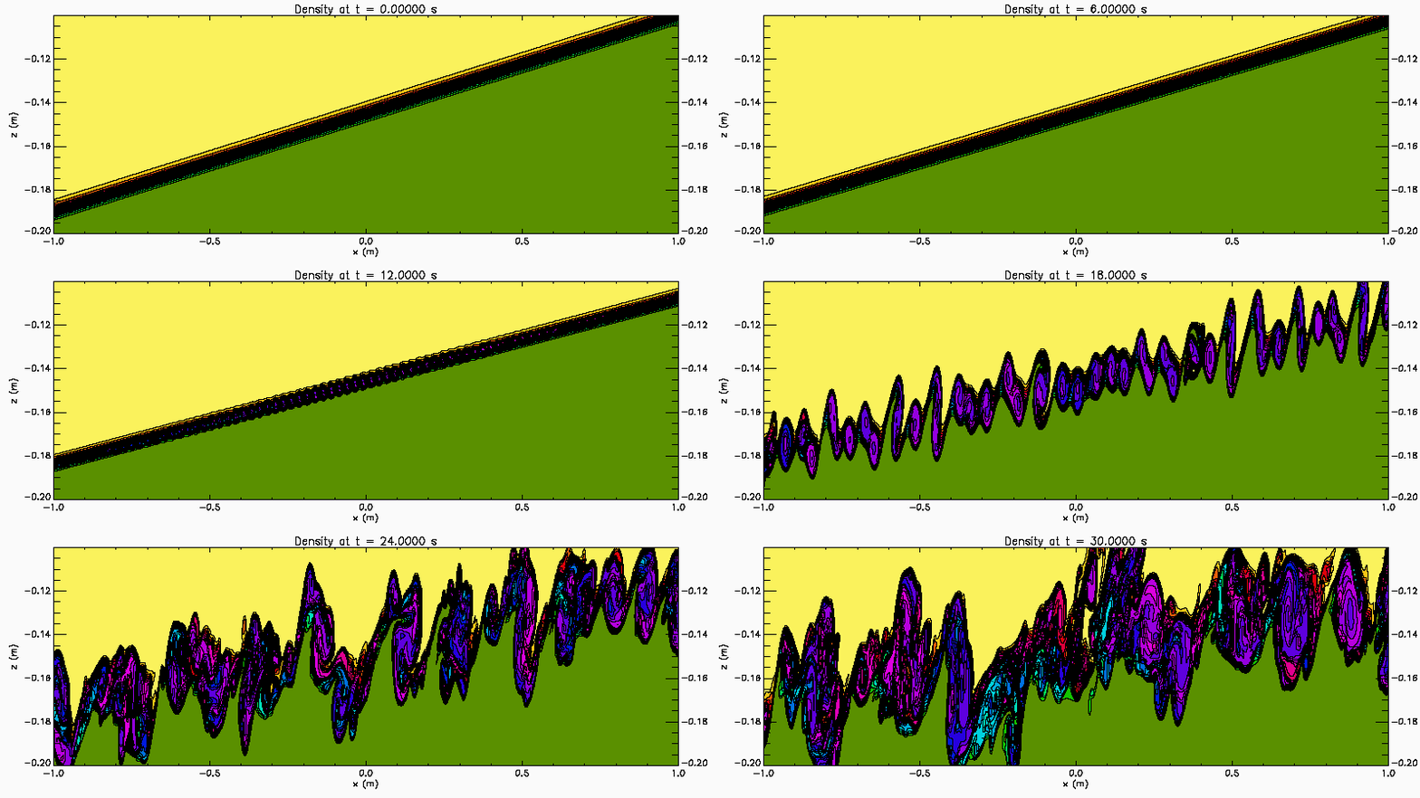
An easy way to generate Kelvin Helmholtz instability in the laboratory is with a tilting tank. Filled with a continuous two-layer stratified water the tank is initial tilted. After the fluid has come to rest the tank is rapidly brought to the horizontal creating an initial stratification with a sloping pycnocline. The baroclinic adjustment creates a sheared flow across the pycnocline. If the initial pycnocline slope is large enough the shear is strong enough to destabilize the flow. This process is illustrated in this numerical simulation which also illustrates the merger of KH billows. In this simulation the tank is 6 m long and 30 cm deep (-3 < x < 3 and -0.3 < z < 0) . The animation shows a section in the central portion of the tank (-1 < x < 1 and -0.2 < z < -0.1).
Kelvin Helmholtz instability
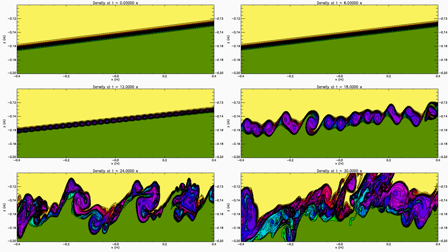
A zoom in of the previous simulation, showing a smaller part of the tank (-0.4 < x < 0.4 and -0.2 < z < -0.1). This provides a closer look at the vortex pairing that occurs.
Spatial instability in an internal solitary wave

This shows the results of a 2D-simulations of a shear instability in an internal solitary wave. The stratification consists of two sharp pycnoclines embedded in a broader pycnocline based on observations on the Oregon Shelf. Wave is propagating to the left through the fluid and the simulation is done in a reference frame moving with the wave. A short pulse perturbation is added in front of the wave. It is advected in the wave where it goes unstable in the upper sharp pycnocline. The minimum Richardson number in the pycnocline is 0.09 at the centre of the wave in the upper sharp pycnocline.
Eigenvalues for Narrow pycnocline: Case 1
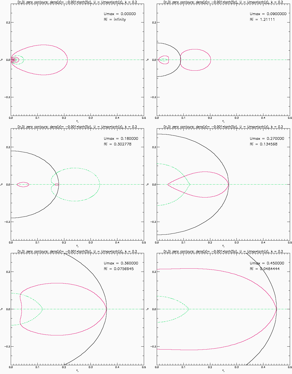
This shows the eigenvalues predicted by linear temporal instability for an inviscid, parallel, stratified shear layer. The background flow is U(z) = Umax*tanh(z) and the background density is rho(z) = 1-0.001*tanh(5z). The vertical domain is -10 <= z <= 10 with solid boundaries. The shear layer is five times thicker than the stratified layer and the Richardson number has its maximum value at the centre of the shear layer. The red and green curves are the zero contours of the real and imaginary parts of the eigenfunction at the top boundary (it is integrated up from the lower boundary). The eigenvalues are found where the red and green curves intersect. The black curve is the circle cr^2+ci^2=Umax^2 of Howard's semi-circle theorem. Unstable modes (and the stable, decaying complex conjugates) must lie inside this circle. The results shown here are for horizonal wave number k=0.2. The eigenvalues are symmetric about the imaginary and the real axis. Only values to the right of the imaginary axis are shown.
When Umax=0 there is no shear flow. The eigenvalues are real and they correspond to the different internal gravity wave modes. The resolution (201x201 grid) can only resolve a finite number of the countable infinity of eigenmodes. As Umax increases they mode 1 wave (largest propagation speed cr) slowly decreases while the others disappear (perhaps a resolution problem). A closed red curve appears inside the black circle (e.g., at Umax = 0.0925). These modes have cr = U(z) at some value of z and hence would have a critical layer. At about Umax = 0.1725 the gravest mode crosses into the black circle and a closed green curve appears. At something like Umax = 0.19 (poorly resolved) the red curve intersects this green curve and there are now a pair of eigenvalues off the real axis. This is Holmboe instability. The move away from the real axis and approach the imaginary axis as Umax continues to increase. The imaginary axis is reached at Umax just above 0.37 at which point they bifurcate and split into two modes, moving up and down the imaginary axis (recall the eigenvalues are symmetric about the imaginary axis). Now the instability is a Kelvin-Helmholtz instability. The mode moving down the imaginary axis reaches the origin at Umax = 0.4475 and then disappears.
Eigenvalues for stratified shear layer: Case 2
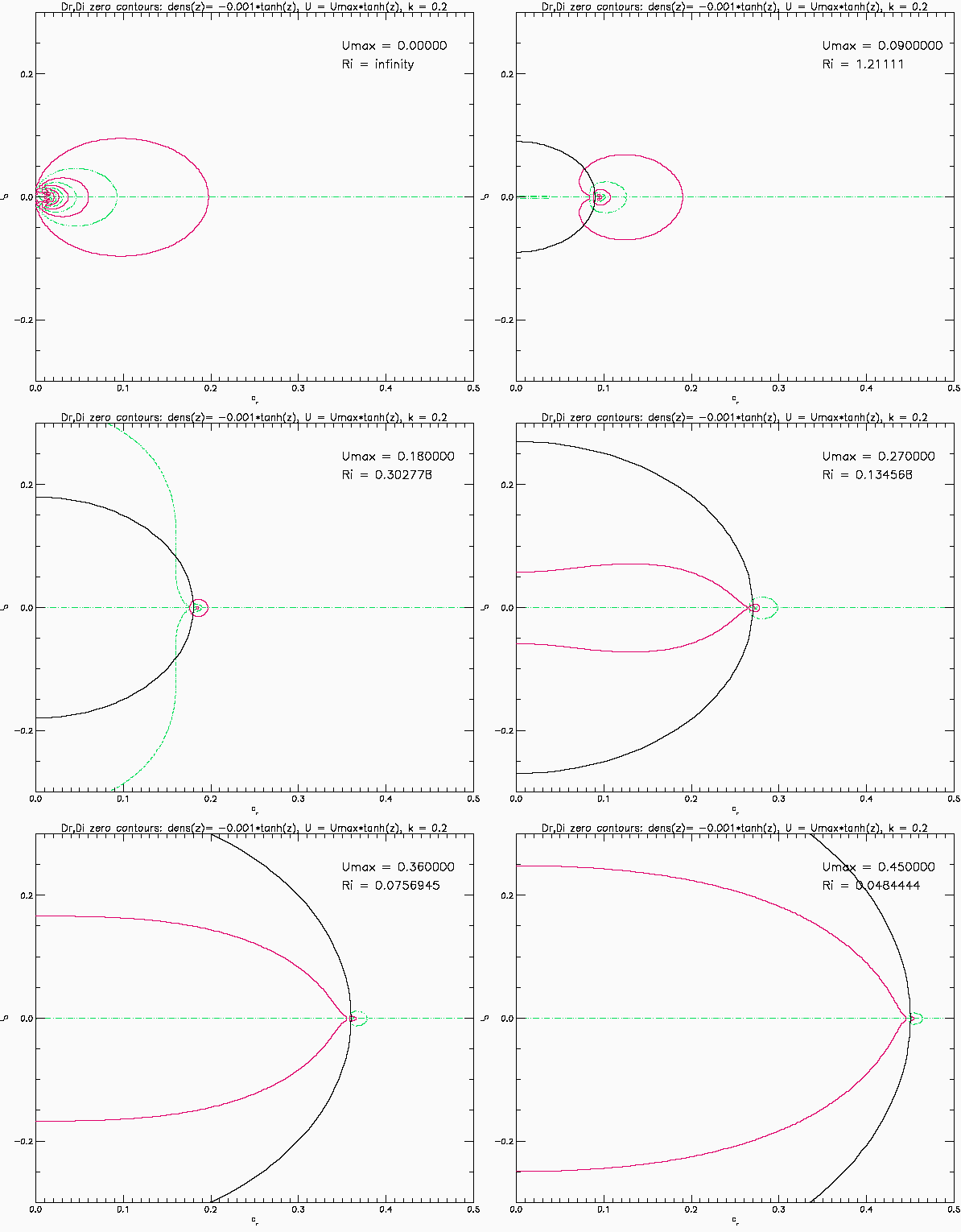
This shows the eigenvalues predicted by linear temporal instability for an inviscid, parallel, stratified shear layer. Same as above but now the shear layer and pycnocline have the same thickness: the background flow is U(z) = Umax*tanh(z) and the background density is rho(z) = 1-0.001*tanh(z). The vertical domain is -10 <= z <= 10 with solid boundaries. The Richardson number now has a minimum at the centre of the shear layer. In this case the eigenvalues stay on the real axis until an eigenvalue reaches the origin at Umax slightly above 0.2425 after which a bifurcation occurs and a pair of eigenmodes move up and down the imaginary axis. The flow is now unstable with stationary eigenmodes. This is Kelvin-Helmoltz instability.
Narrow pycnocline: Case 1
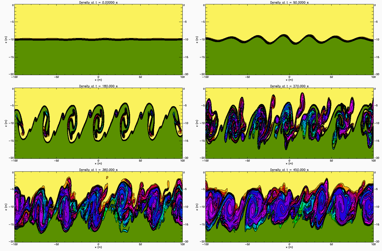
This shows the results of a 2D-simulations of a stratified shear instability. The background flow is U(z) = 0.38*tanh(z). The background density is rho(z) = 1-0.001*tanh(5z). The shear layer is five times thicker than the stratified layer and the Richardson number has a maximum value of 0.34 at the centre of the shear layer. In this similation the flow is initialized with a density perturbation with wave number 0.2, modulated by a sech(x/100.0) envelope. Domain is -20 <= z <= 0 with solid boundaries. Linear temporal stability theory predicts a pair of unstable eigenmode with phase speeds c1 = 0.121i and c2 = 0.121i. Because there is a pair of unstable waves propagating slowly in opposite directions relative to the centre of the shear layer weak characteristics of a Holmboe Instability.
Narrow pycnocline: Case 2

Same as preceeding case but with U(z) = 0.35*tanh(z). The Richardson number now has a maximum value of 0.40 at the centre of the shear layer. Linear temporal stability theory predicts a pair of unstable eigenmode with phase speeds c1 = 0.051+0.077i and c2 = -0.051+0.077i. Because there is a pair of unstable waves propagating slowly in opposite directions relative to the centre of the shear layer the instability has weak characteristics of a Holmboe Instability.
Narrow pycnocline: Case 3
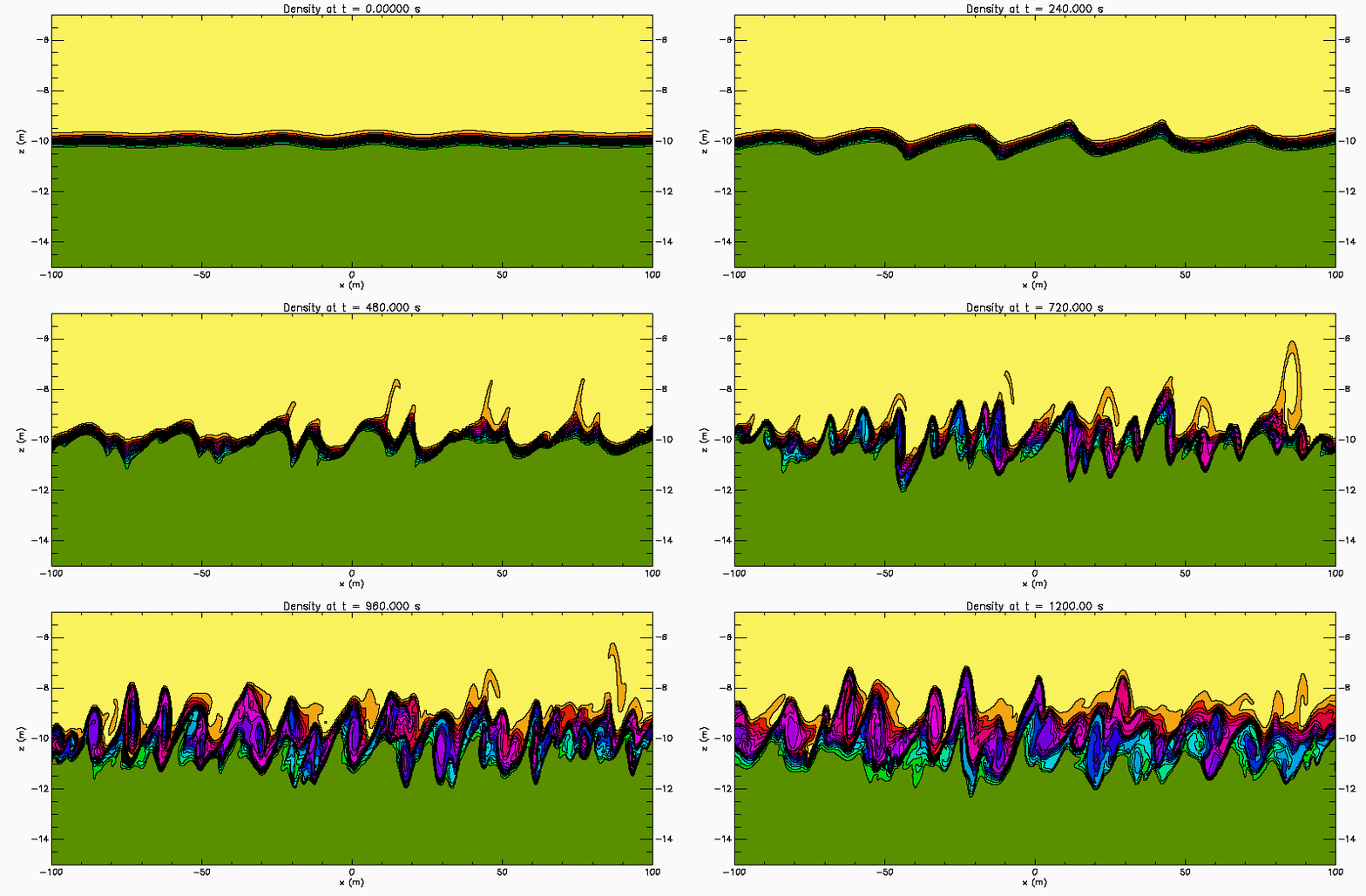
Same as preceeding case but with U(z) = 0.22*tanh(z). The Richardson number has a maximum value of 1.01 at the centre of the shear layer. Linear stability theory predicts a pair of unstable eigenmodes with phase speed c1 = 0.130+0.010i and c2 = -0.130+0.010i. In this case the instability more clearly illustrates the Holmboe Instability. Because of the small growth of the perturbation the animation zooms into the region -15 <= z <= -5.
Narrow pycnocline: Case 4

Same as preceeding case but with U(z) = 0.21*tanh(z). The Richardson number has a maximum value of 1.11 at the centre of the shear layer. Linear stability theory predicts a pair of unstable eigenmodes with phase speed c1 = 0.141+0.004i and c2 = -0.141+0.004i. In this case the instability more clearly illustrates the Holmboe Instability. Because of the small growth of the perturbation the animation zooms into the region -15 <= z <= -5.
Convective instability in two layer fluid
This shows the results of a 2D-simulations of convective instability. The initial stratification has dense fluid over light fluid with sinusoidal perturbations to the pycnocline modulated by a sech squared envelope. Upper and lower layer densities are 1010 and 990 kg/m^3. Kinematic viscosity 0.0002 m^2/s. Diffusivity 0.00001 m^2/s. Tank is 1m by 0.3m. No-slip boundary conditions used along top, bottom and sides. Large (10MB gif file).
Same as preceeding case but initial perturbation is a single sech squared depression. (Long (10MB gif file)) (Short (6MB gif file))
Same as preceeding case but viscosity and diffusivity both decreased by a factor of 10. (Long(12MB gif file)) (Short (6MB gif file)) (Small (2MB gif file))
Viscosity and diffusivity reduced even further to 1.0e-6 m^2/s and 1.0e-7 m^2/6. (Long (15MB gif file)) (Short (6MB gif file))
Parametric subharmonic instability
Parametric subharmonic instability (PSI) involves the transfer of energy to frequencies of approximately half the frequency of the primary wave. This numerical simulation was initialized with a linear internal standing wave in a closed basin. Perturbations are generated by the nonlinear terms. Ultimately a perturbation of half the frequency of the initial wave grows. From 2D-simulation. (9MB gif file) (Small (5MB gif file))
Multi-layer flows: Dispersion curves
Two layer gravity-capillary waves (0.6MB gif file): This is an animation of the dispersion curves (frequency vs wave number) for 2-D waves on the air-water interface as the wind speed varies. Water is at rest. Both layers are infinitely deep. For a critical value of the air speed (just above 6.5 m/s) a gap appears in the dispersion curves in which the flow is unstable. Long wave (small k) are stabilized by gravity and short waves (large k) are stabilized by surface tension.
Two layer gravity-capillary waves (0.6MB gif file): As above but now in a reference frame in which the water is moving with velocity 0.1 m/s to the right.
Three-layer flow (1.06MB gif file): This is an animation of the dispersion curves for the three layer flow considered by Adam & Craik (1979). See text by Craik as well. The upper, middle and lower layers have densities of 1015, 1020 and 1026 kg/m^3 respectively. Surface tension of 0.074 N/m acts on the upper interface. The surface tension on the lower interface is taken to be zero. The upper and lower layers are infinitely deep while the middle layer is 16 cm thick. The lower and middle layers are at rest. The dispersion curves (frequency vs horizontal wave number) vary as U1, the current in the upper layer, is increased from zero. When U1 = 0 an exchange of identities between lower branches of the gravity waves on the lower interface and the gravity-capillary waves on the upper interface can be seen near k=15 1/m. A similar exchange of identities occurs between the upper branches. As U1 increases the value of k at which the exchange occurs moves off to the right and the two curves get closer and closer together. Then never intersect. The dispersion curves corresponding to the gravity-capillary waves on the upper interface both move up. The lower branch eventually crosses the sigma-axis and approaches the upper branch of the gravity wave curve. These two curves coalesce and gaps appear in which the flow is unstable. After the lower gravity-capillary wave branch passes through the upper gravity wave branch the two gravity-capillary wave branches approach each other (with the upper one now moving down) until they too coalesce forming and new unstable wave number band.
Three-layer flow (1.06MB gif file): This is the same as the above but with dispersion curves for gravity-capillary waves on the upper interface (green curve) and for gravity waves on the lower interface (blue curve) included for comparison. These additional dispersion curves are those for two layer flows, both layers infinitely deep.